NASA Earthdata Access in the Cloud Using Open-source libraries
Contributing co-authors
Catalina M Oaida; NASA PO.DAAC, NASA JPL
Luis Alberto Lopez; NASA National Snow and Ice Data Center DAAC
Aaron Friesz; NASA Land Processes DAAC
Andrew P Barrett; NASA National Snow and Ice Data Center DAAC
Makhan Virdi; NASA ASDC DAAC
Jack McNelis; NASA PO.DAAC, NASA JPL
Julia Lowndes; Openscapes, NCEAS
Erin Robinson; Openscapes, Metadata Game Changers
Additional thanks to the entire NASA Earthdata Openscapes community, Patrick Quinn at Element84, and to 2i2c for our Cloud infrastructure.
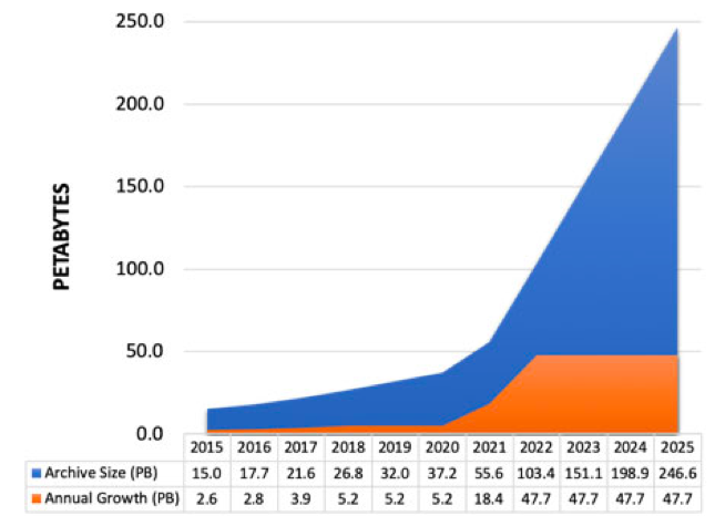
NASA Earthdata archive growth

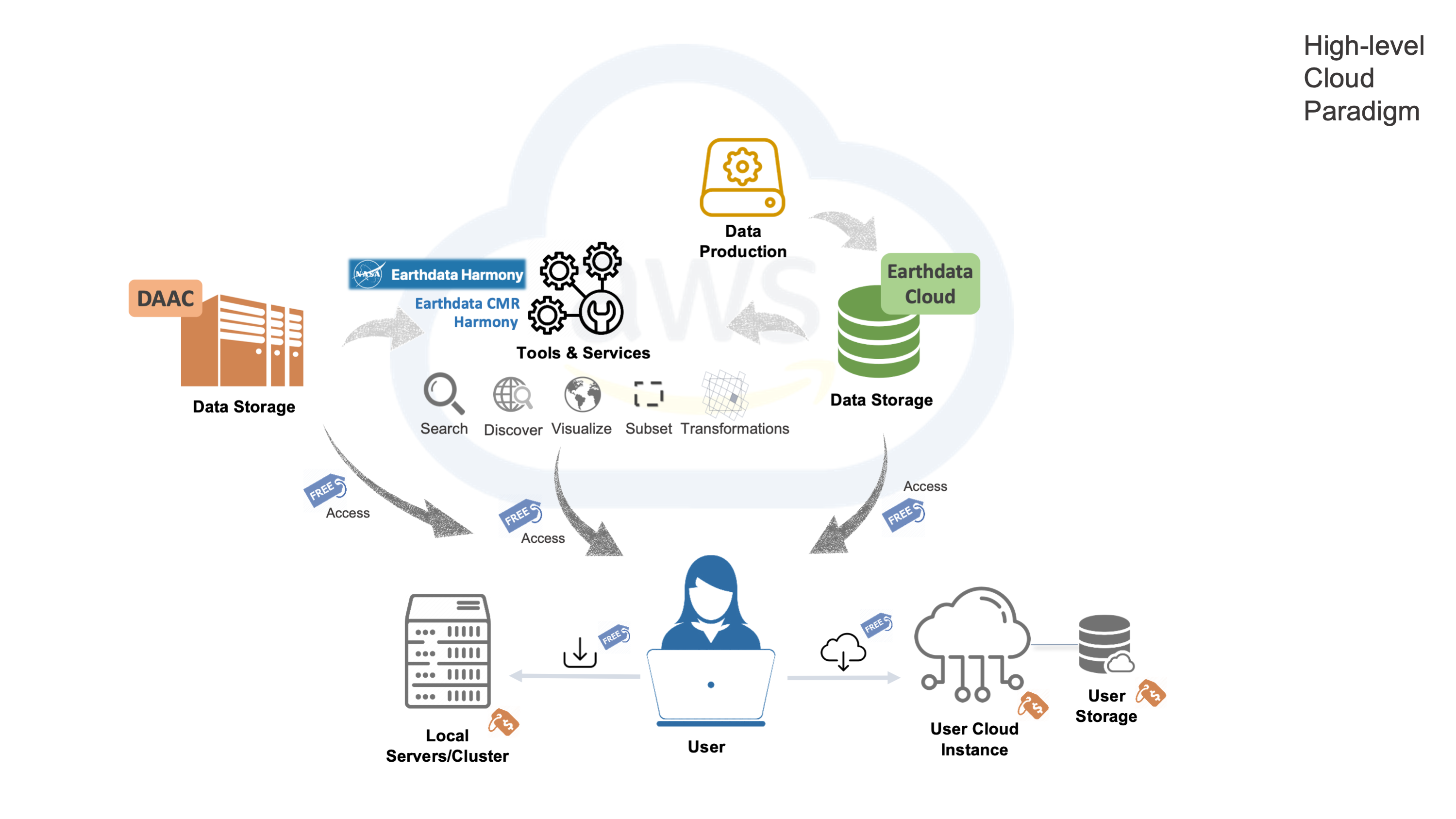
The NASA Earthdata Cloud Evolution
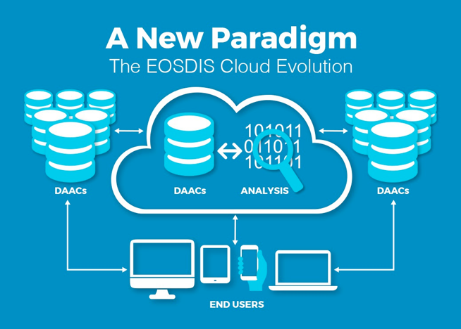
NASA Distributed Active Archive Centers (DAACs) are continuing to migrate data to the Earthdata Cloud
- Supporting increased data volume as new, high-resolution remote sensing missions launch in the coming years
- Data hosted via Amazon Web Services, or AWS
- DAACs continuing to support tools, services, and tutorial resources for our user communities
Part 1: Explore Earthdata Cloud
Earthdata Search Demo
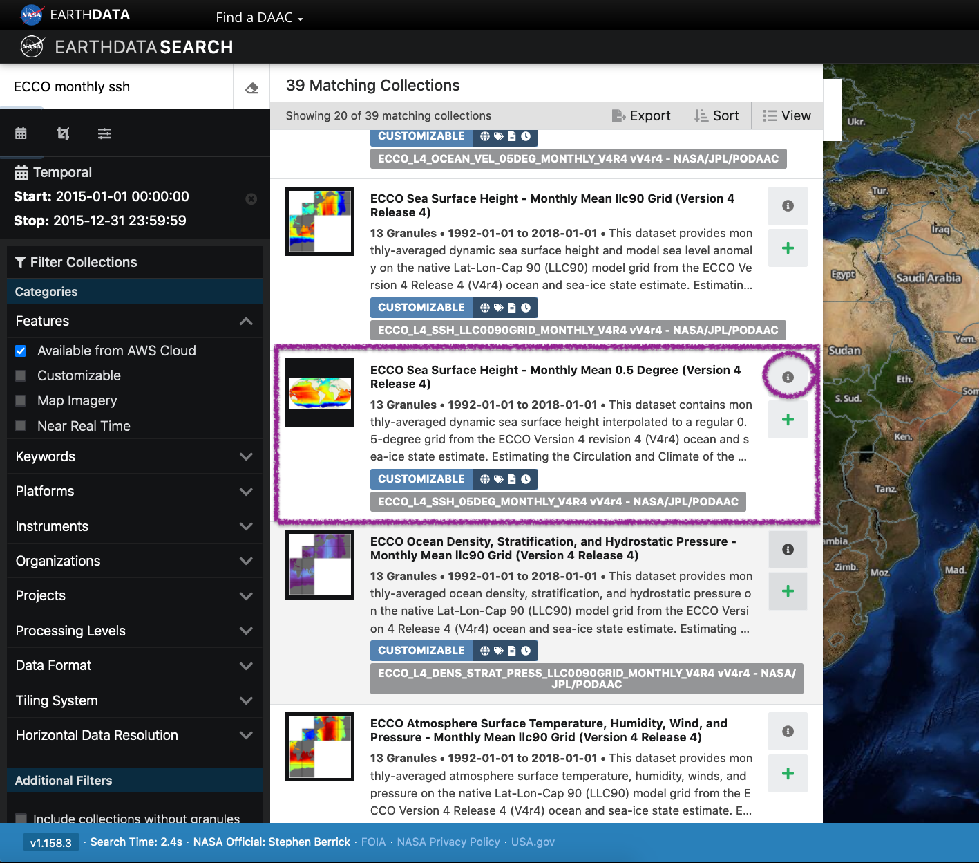
The “Available from AWS Cloud” filter option returns all data from the NASA Earthdata Cloud, including the ECCO dataset, hosted by the PO.DAAC. Here, we search for ECCO monthly SSH over the time period for the year 2015.
View and Select Data Access Options
Clicking on the ECCO Sea Surface Height - Monthly Mean 0.5 Degree (Version 4 Release 4) dataset provides a list of files (granules) that are part of the dataset (collection). There we can select files to add to our project, with options to customize our download or access link(s).
Earthdata Search: Access Options
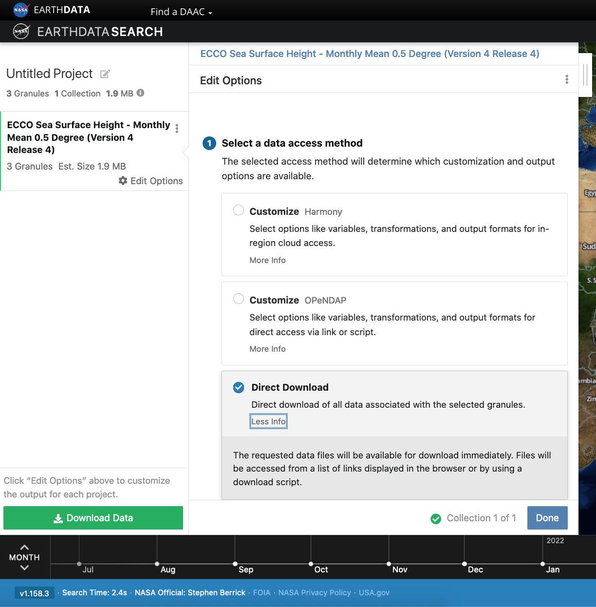
Select the “Direct Download” option to view Access options via Direct Download and from the AWS Cloud. Additional options to customize the data are also available for this dataset.
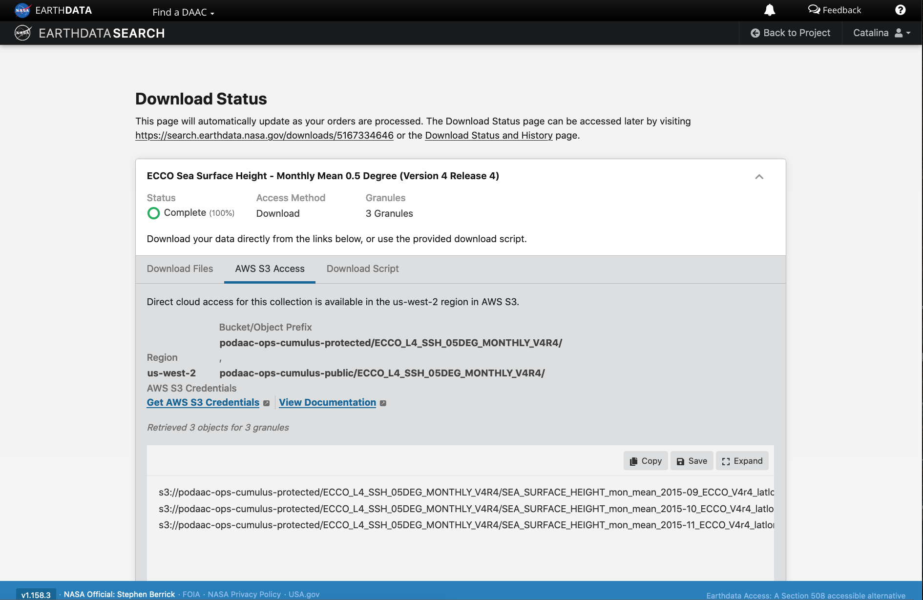
Earthdata Cloud access information
The final ordering page provides instructions to download and links for data access in the cloud. The AWS S3 Access tab provides the S3:// links, which is what we would use to access the data directly in-region (us-west-2) within the AWS cloud. E.g.: s3://podaac-ops-cumulus-protected/ECCO_L4_SSH_05DEG_MONTHLY_V4R4/SEA_SURFACE_HEIGHT_mon_mean_2015-09_ECCO_V4r4_latlon_0p50deg.nc where s3 indicates data is stored in AWS S3 storage, podaac-ops-cumulus-protected is the bucket, and ECCO_L4_SSH_05DEG_MONTHLY_V4R4 is the object prefix (the latter two are also listed in the dataset collection information under Cloud Access (step 3 above)).
Earthdata Cloud access information
Integrate file links into programmatic workflow, locally or in the AWS cloud.
We can connect these access links to subsequent data analysis in the cloud by either copy/pasting the s3:// links or saving them as a text file to then access in a Jupyter notebook or script running in the cloud.
Search for STAC Items: Read in a geojson file and plot
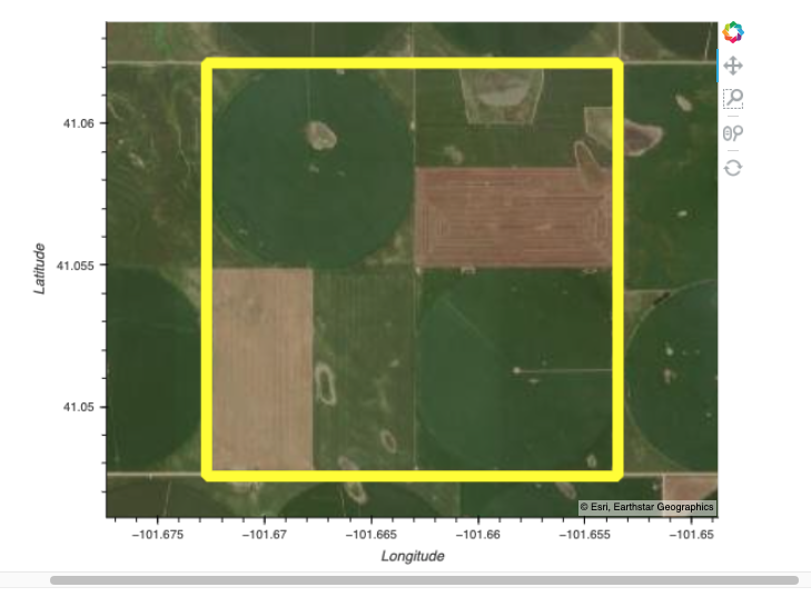
We will define our ROI using a geojson file containing a small polygon feature in western Nebraska, USA. We’ll also specify the data collections and a time range for our example.
Read in a geojson file with geopandas and extract coodinates for our ROI. We can plot the polygon using the geoviews package that we imported as gv with ‘bokeh’ and ‘matplotlib’ extensions. The following has reasonable width, height, color, and line widths to view our polygon when it is overlayed on a base tile map.
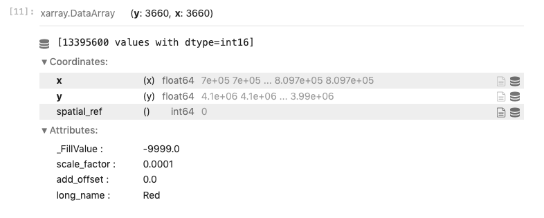
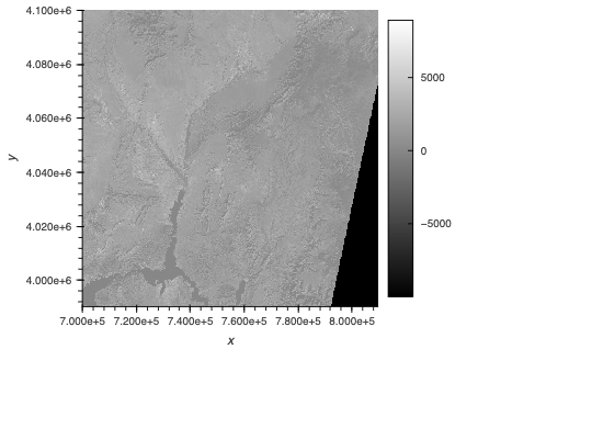
Read Cloud-Optimized GeoTIFF into rioxarray
Plot using hvplot
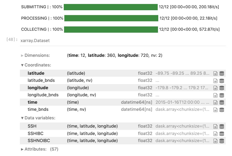
Open staged files with s3fs and xarray
Open the Zarr stores using the s3fs package, then load them all at once into a concatenated xarray dataset:
Plot the Sea Surface Height time series using hvplot
Now we can start looking at aggregations across the time dimension. Here we plot the SSH variable using hvplot and can use the time slider to visualize changes in SSH over the year.

Data and Analysis co-located “in place”
NASA Earthdata Cloud as an enabler of Open Science

*Reducing barriers to large-scale scientific research in the era of “big data”
*Increasing community contributions with hands-on engagement
*Promoting reproducible and shareable workflows without relying on local storage systems
Building NASA Earthdata Cloud Resources
