Using icepyx to access ICESat-2 data

!pip install icepyx==0.8.1 -qq

What is icepyx?

icepyx is a community and software library for searching, downloading, and reading ICESat-2 data. While opening data should be straightforward, there are some oddities in navigating the highly nested organization and hundreds of variables of the ICESat-2 data. icepyx provides tools to help with those oddities.

Fitting icepyx into the data access package landscape

For ICESat-2 data, the icepyx package can: - search for available data granules (data files) - order and download data - order a subset of data: clipped in space, time, containing fewer variables, or a few other options provided by NSIDC - provides functionality to search through the available data variables - read ICESat-2 data into xarray DataArrays, including merging data from multiple files

What is ICESat-2?

IS2

ICESat-2 carries a satellite lidar instrument, ATLAS. Lidar is an active remote sensing technique in which pulses of light are emitted and the return time is used to measure distance. The available ICESat-2 data products range from sea ice freeboard to land elevation to cloud backscatter characteristics. A list of availble products can be found here. In this tutorial we will look at the ATL08 Land Water Vegetation Elevation product.

Data Collection

ICESat-2 measures data along 3 strong/weak beam pairs, resulting in 3 strong beams and 3 weak beams. The strong and weak beams are calibrated such that the weak beams have more sensitivity to viewing very bright surfaces (Ex. ice), while the strong beams are able to view surfaces with lower reflectances (Ex. water). The beams are designated in each data product as gt1l, gt1r, gt2l, gt2r, gt3l, and gt3r, where gt stands for “ground track”, the number refers to the photon emitter, and the l and r indicate “left” or “right” beam of the pair. Which of these designations is strong or weak depends on the orientation of the satellite (forwards, sc_orient==1; backwards, sc_orient==0). A helpful table of which beams are strong/weak can be found on p131 of the ATL03 Algorithm Theoretical Basis Document. The ATLAS spot number (values 1-6) is based on the ground track designation (gt1l etc.) and spacecraft orientation and, once determined can be used to consistently identify strong (Spots 1, 3, and 5) and weak (Spots 2, 4, and 6) beams.

Tracks

Photo: Neuenschwander et. al. 2019, Remote Sens. Env. DOI

Counting Photons

The ICESat-2 lidar collects at the single photon level, different from most commercial lidar systems. A lot of additional photons get returned as solar background noise, and removing these unwanted photons is a key part of the algorithms that produce the higher level data products.

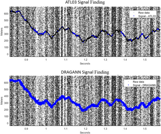
Fig. 2. Results from signal finding methods for simulated ATLAS data. Black points show raw point cloud data as ingested from ATL03 product. Blue points overlaid in each plot show which photons each method identified as signal. Top panel reflects the signal photons as identified on the ATL03 data product (medium and high confidence signal photons). Bottom panel reflects the signal photons identified from the ATL08 DRAGANN method. (Neuenschwander & Pitts, 2019)

Photo: Neuenschwander et. al. 2019, Remote Sens. Env. DOI

To aggregate all these photons into more manegable chunks ATL08 consolidates the photons into 100m segments, each made up of five 20m segments.

Using icepyx to search for data

We won’t dive into using icepyx to search for and download data in this tutorial, since we already discussed how to do that with earthaccess. The code to search and download is still provided below for the curious reader. The icepyx documentation shows more detail about different search parameters and how to inspect the results of a query.

import icepyx as ipx

import json
import math

import numpy as np
import matplotlib.pyplot as plt
from shapely.geometry import shape, GeometryCollection

%matplotlib inline

# Open a geojson of our area of interest
with open("bosque_primavera.json") as f:
    features = json.load(f)["features"]

bosque = GeometryCollection([shape(feature["geometry"]).buffer(0) for feature in features])

# Use our search parameters to setup a search Query
short_name = 'ATL08'
spatial_extent = list(bosque.bounds)
date_range = ['2019-05-04','2019-05-04']
region = ipx.Query(short_name, spatial_extent, date_range)

# Display if any data files, or granules, matched our search
region.avail_granules(ids=True)

[['ATL08_20190504124152_05540301_006_02.h5']]

# Download the granules to a into a folder called 'bosque_primavera_ATL08'
region.download_granules('./bosque_primavera_ATL08')

EARTHDATA_USERNAME and EARTHDATA_PASSWORD are not set in the current environment, try setting them or use a different strategy (netrc, interactive)
You're now authenticated with NASA Earthdata Login
Using token with expiration date: 12/15/2023
Using .netrc file for EDL
Total number of data order requests is  1  for  1  granules.
Data request  1  of  1  is submitting to NSIDC
order ID:  5000004610385
Initial status of your order request at NSIDC is:  processing
Your order status is still  processing  at NSIDC. Please continue waiting... this may take a few moments.
Your order is: complete
Beginning download of zipped output...
Data request 5000004610385 of  1  order(s) is downloaded.
Download complete

Tip: If you don’t want to type your earthdata login information every time they are required you can setup more automatic methods of authentication. Two common methods are 1) Add your earthdata password and username to as environment variables as EARTHDATA_USERNAME and EARTHDATA_PASSWORD. 2) setup a .netrc file in your home directory. See the Openscapes tutorial

Reading a file with icepyx

To read a file with icepyx there are several steps: 1. Create a Read object. This sets up an initial connection to your file(s) and validates the metadata. 2. Tell the Read object what variables you would like to read 3. Load your data!

Create a Read object

pattern = "processed_ATL{product:2}_{datetime:%Y%m%d%H%M%S}_{rgt:4}{cycle:2}{orbitsegment:2}_{version:3}_{revision:2}.h5"
reader = ipx.Read('./bosque_primavera_ATL08', "ATL08", pattern)

You have 1 files matching the filename pattern to be read in.

reader

<icepyx.core.read.Read at 0x7f3d05e72e90>

Select your variables

To view the variables contained in your dataset you can call .vars on your data reader.

reader.vars.avail()

['ancillary_data/atlas_sdp_gps_epoch',
 'ancillary_data/control',
 'ancillary_data/data_end_utc',
 'ancillary_data/data_start_utc',
 'ancillary_data/end_cycle',
 'ancillary_data/end_delta_time',
 'ancillary_data/end_geoseg',
 'ancillary_data/end_gpssow',
 'ancillary_data/end_gpsweek',
 'ancillary_data/end_orbit',
 'ancillary_data/end_region',
 'ancillary_data/end_rgt',
 'ancillary_data/granule_end_utc',
 'ancillary_data/granule_start_utc',
 'ancillary_data/land/atl08_region',
 'ancillary_data/land/bin_size_h',
 'ancillary_data/land/bin_size_n',
 'ancillary_data/land/bright_thresh',
 'ancillary_data/land/ca_class',
 'ancillary_data/land/can_noise_thresh',
 'ancillary_data/land/can_stat_thresh',
 'ancillary_data/land/canopy20m_thresh',
 'ancillary_data/land/canopy_flag_switch',
 'ancillary_data/land/canopy_seg',
 'ancillary_data/land/class_thresh',
 'ancillary_data/land/cloud_filter_switch',
 'ancillary_data/land/del_amp',
 'ancillary_data/land/del_mu',
 'ancillary_data/land/del_sigma',
 'ancillary_data/land/dem_filter_switch',
 'ancillary_data/land/dem_removal_percent_limit',
 'ancillary_data/land/dragann_switch',
 'ancillary_data/land/dseg',
 'ancillary_data/land/dseg_buf',
 'ancillary_data/land/fnlgnd_filter_switch',
 'ancillary_data/land/gnd_stat_thresh',
 'ancillary_data/land/gthresh_factor',
 'ancillary_data/land/h_canopy_perc',
 'ancillary_data/land/iter_gnd',
 'ancillary_data/land/iter_max',
 'ancillary_data/land/lseg',
 'ancillary_data/land/lseg_buf',
 'ancillary_data/land/lw_filt_bnd',
 'ancillary_data/land/lw_gnd_bnd',
 'ancillary_data/land/lw_toc_bnd',
 'ancillary_data/land/lw_toc_cut',
 'ancillary_data/land/max_atl03files',
 'ancillary_data/land/max_atl09files',
 'ancillary_data/land/max_peaks',
 'ancillary_data/land/max_try',
 'ancillary_data/land/min_nphs',
 'ancillary_data/land/n_dec_mode',
 'ancillary_data/land/night_thresh',
 'ancillary_data/land/noise_class',
 'ancillary_data/land/outlier_filter_switch',
 'ancillary_data/land/p_static',
 'ancillary_data/land/ph_removal_percent_limit',
 'ancillary_data/land/proc_geoseg',
 'ancillary_data/land/psf',
 'ancillary_data/land/ref_dem_limit',
 'ancillary_data/land/ref_finalground_limit',
 'ancillary_data/land/relief_hbot',
 'ancillary_data/land/relief_htop',
 'ancillary_data/land/shp_param',
 'ancillary_data/land/sig_rsq_search',
 'ancillary_data/land/sseg',
 'ancillary_data/land/stat20m_thresh',
 'ancillary_data/land/stat_thresh',
 'ancillary_data/land/tc_thresh',
 'ancillary_data/land/te_class',
 'ancillary_data/land/terrain20m_thresh',
 'ancillary_data/land/toc_class',
 'ancillary_data/land/up_filt_bnd',
 'ancillary_data/land/up_gnd_bnd',
 'ancillary_data/land/up_toc_bnd',
 'ancillary_data/land/up_toc_cut',
 'ancillary_data/land/yapc_switch',
 'ancillary_data/qa_at_interval',
 'ancillary_data/release',
 'ancillary_data/start_cycle',
 'ancillary_data/start_delta_time',
 'ancillary_data/start_geoseg',
 'ancillary_data/start_gpssow',
 'ancillary_data/start_gpsweek',
 'ancillary_data/start_orbit',
 'ancillary_data/start_region',
 'ancillary_data/start_rgt',
 'ancillary_data/version',
 'ds_geosegments',
 'ds_metrics',
 'ds_surf_type',
 'gt3l/land_segments/asr',
 'gt3l/land_segments/atlas_pa',
 'gt3l/land_segments/beam_azimuth',
 'gt3l/land_segments/beam_coelev',
 'gt3l/land_segments/brightness_flag',
 'gt3l/land_segments/canopy/can_noise',
 'gt3l/land_segments/canopy/canopy_h_metrics',
 'gt3l/land_segments/canopy/canopy_h_metrics_abs',
 'gt3l/land_segments/canopy/canopy_openness',
 'gt3l/land_segments/canopy/canopy_rh_conf',
 'gt3l/land_segments/canopy/centroid_height',
 'gt3l/land_segments/canopy/h_canopy',
 'gt3l/land_segments/canopy/h_canopy_20m',
 'gt3l/land_segments/canopy/h_canopy_abs',
 'gt3l/land_segments/canopy/h_canopy_quad',
 'gt3l/land_segments/canopy/h_canopy_uncertainty',
 'gt3l/land_segments/canopy/h_dif_canopy',
 'gt3l/land_segments/canopy/h_max_canopy',
 'gt3l/land_segments/canopy/h_max_canopy_abs',
 'gt3l/land_segments/canopy/h_mean_canopy',
 'gt3l/land_segments/canopy/h_mean_canopy_abs',
 'gt3l/land_segments/canopy/h_median_canopy',
 'gt3l/land_segments/canopy/h_median_canopy_abs',
 'gt3l/land_segments/canopy/h_min_canopy',
 'gt3l/land_segments/canopy/h_min_canopy_abs',
 'gt3l/land_segments/canopy/n_ca_photons',
 'gt3l/land_segments/canopy/n_toc_photons',
 'gt3l/land_segments/canopy/photon_rate_can',
 'gt3l/land_segments/canopy/photon_rate_can_nr',
 'gt3l/land_segments/canopy/segment_cover',
 'gt3l/land_segments/canopy/subset_can_flag',
 'gt3l/land_segments/canopy/toc_roughness',
 'gt3l/land_segments/cloud_flag_atm',
 'gt3l/land_segments/cloud_fold_flag',
 'gt3l/land_segments/delta_time',
 'gt3l/land_segments/delta_time_beg',
 'gt3l/land_segments/delta_time_end',
 'gt3l/land_segments/dem_flag',
 'gt3l/land_segments/dem_h',
 'gt3l/land_segments/dem_removal_flag',
 'gt3l/land_segments/h_dif_ref',
 'gt3l/land_segments/last_seg_extend',
 'gt3l/land_segments/latitude',
 'gt3l/land_segments/latitude_20m',
 'gt3l/land_segments/layer_flag',
 'gt3l/land_segments/longitude',
 'gt3l/land_segments/longitude_20m',
 'gt3l/land_segments/msw_flag',
 'gt3l/land_segments/n_seg_ph',
 'gt3l/land_segments/night_flag',
 'gt3l/land_segments/ph_ndx_beg',
 'gt3l/land_segments/ph_removal_flag',
 'gt3l/land_segments/psf_flag',
 'gt3l/land_segments/rgt',
 'gt3l/land_segments/sat_flag',
 'gt3l/land_segments/segment_id_beg',
 'gt3l/land_segments/segment_id_end',
 'gt3l/land_segments/segment_landcover',
 'gt3l/land_segments/segment_snowcover',
 'gt3l/land_segments/segment_watermask',
 'gt3l/land_segments/sigma_across',
 'gt3l/land_segments/sigma_along',
 'gt3l/land_segments/sigma_atlas_land',
 'gt3l/land_segments/sigma_h',
 'gt3l/land_segments/sigma_topo',
 'gt3l/land_segments/snr',
 'gt3l/land_segments/solar_azimuth',
 'gt3l/land_segments/solar_elevation',
 'gt3l/land_segments/surf_type',
 'gt3l/land_segments/terrain/h_te_best_fit',
 'gt3l/land_segments/terrain/h_te_best_fit_20m',
 'gt3l/land_segments/terrain/h_te_interp',
 'gt3l/land_segments/terrain/h_te_max',
 'gt3l/land_segments/terrain/h_te_mean',
 'gt3l/land_segments/terrain/h_te_median',
 'gt3l/land_segments/terrain/h_te_min',
 'gt3l/land_segments/terrain/h_te_mode',
 'gt3l/land_segments/terrain/h_te_rh25',
 'gt3l/land_segments/terrain/h_te_skew',
 'gt3l/land_segments/terrain/h_te_std',
 'gt3l/land_segments/terrain/h_te_uncertainty',
 'gt3l/land_segments/terrain/n_te_photons',
 'gt3l/land_segments/terrain/photon_rate_te',
 'gt3l/land_segments/terrain/subset_te_flag',
 'gt3l/land_segments/terrain/terrain_slope',
 'gt3l/land_segments/terrain_flg',
 'gt3l/land_segments/urban_flag',
 'gt3l/signal_photons/classed_pc_flag',
 'gt3l/signal_photons/classed_pc_indx',
 'gt3l/signal_photons/d_flag',
 'gt3l/signal_photons/delta_time',
 'gt3l/signal_photons/ph_h',
 'gt3l/signal_photons/ph_segment_id',
 'gt3r/land_segments/asr',
 'gt3r/land_segments/atlas_pa',
 'gt3r/land_segments/beam_azimuth',
 'gt3r/land_segments/beam_coelev',
 'gt3r/land_segments/brightness_flag',
 'gt3r/land_segments/canopy/can_noise',
 'gt3r/land_segments/canopy/canopy_h_metrics',
 'gt3r/land_segments/canopy/canopy_h_metrics_abs',
 'gt3r/land_segments/canopy/canopy_openness',
 'gt3r/land_segments/canopy/canopy_rh_conf',
 'gt3r/land_segments/canopy/centroid_height',
 'gt3r/land_segments/canopy/h_canopy',
 'gt3r/land_segments/canopy/h_canopy_20m',
 'gt3r/land_segments/canopy/h_canopy_abs',
 'gt3r/land_segments/canopy/h_canopy_quad',
 'gt3r/land_segments/canopy/h_canopy_uncertainty',
 'gt3r/land_segments/canopy/h_dif_canopy',
 'gt3r/land_segments/canopy/h_max_canopy',
 'gt3r/land_segments/canopy/h_max_canopy_abs',
 'gt3r/land_segments/canopy/h_mean_canopy',
 'gt3r/land_segments/canopy/h_mean_canopy_abs',
 'gt3r/land_segments/canopy/h_median_canopy',
 'gt3r/land_segments/canopy/h_median_canopy_abs',
 'gt3r/land_segments/canopy/h_min_canopy',
 'gt3r/land_segments/canopy/h_min_canopy_abs',
 'gt3r/land_segments/canopy/n_ca_photons',
 'gt3r/land_segments/canopy/n_toc_photons',
 'gt3r/land_segments/canopy/photon_rate_can',
 'gt3r/land_segments/canopy/photon_rate_can_nr',
 'gt3r/land_segments/canopy/segment_cover',
 'gt3r/land_segments/canopy/subset_can_flag',
 'gt3r/land_segments/canopy/toc_roughness',
 'gt3r/land_segments/cloud_flag_atm',
 'gt3r/land_segments/cloud_fold_flag',
 'gt3r/land_segments/delta_time',
 'gt3r/land_segments/delta_time_beg',
 'gt3r/land_segments/delta_time_end',
 'gt3r/land_segments/dem_flag',
 'gt3r/land_segments/dem_h',
 'gt3r/land_segments/dem_removal_flag',
 'gt3r/land_segments/h_dif_ref',
 'gt3r/land_segments/last_seg_extend',
 'gt3r/land_segments/latitude',
 'gt3r/land_segments/latitude_20m',
 'gt3r/land_segments/layer_flag',
 'gt3r/land_segments/longitude',
 'gt3r/land_segments/longitude_20m',
 'gt3r/land_segments/msw_flag',
 'gt3r/land_segments/n_seg_ph',
 'gt3r/land_segments/night_flag',
 'gt3r/land_segments/ph_ndx_beg',
 'gt3r/land_segments/ph_removal_flag',
 'gt3r/land_segments/psf_flag',
 'gt3r/land_segments/rgt',
 'gt3r/land_segments/sat_flag',
 'gt3r/land_segments/segment_id_beg',
 'gt3r/land_segments/segment_id_end',
 'gt3r/land_segments/segment_landcover',
 'gt3r/land_segments/segment_snowcover',
 'gt3r/land_segments/segment_watermask',
 'gt3r/land_segments/sigma_across',
 'gt3r/land_segments/sigma_along',
 'gt3r/land_segments/sigma_atlas_land',
 'gt3r/land_segments/sigma_h',
 'gt3r/land_segments/sigma_topo',
 'gt3r/land_segments/snr',
 'gt3r/land_segments/solar_azimuth',
 'gt3r/land_segments/solar_elevation',
 'gt3r/land_segments/surf_type',
 'gt3r/land_segments/terrain/h_te_best_fit',
 'gt3r/land_segments/terrain/h_te_best_fit_20m',
 'gt3r/land_segments/terrain/h_te_interp',
 'gt3r/land_segments/terrain/h_te_max',
 'gt3r/land_segments/terrain/h_te_mean',
 'gt3r/land_segments/terrain/h_te_median',
 'gt3r/land_segments/terrain/h_te_min',
 'gt3r/land_segments/terrain/h_te_mode',
 'gt3r/land_segments/terrain/h_te_rh25',
 'gt3r/land_segments/terrain/h_te_skew',
 'gt3r/land_segments/terrain/h_te_std',
 'gt3r/land_segments/terrain/h_te_uncertainty',
 'gt3r/land_segments/terrain/n_te_photons',
 'gt3r/land_segments/terrain/photon_rate_te',
 'gt3r/land_segments/terrain/subset_te_flag',
 'gt3r/land_segments/terrain/terrain_slope',
 'gt3r/land_segments/terrain_flg',
 'gt3r/land_segments/urban_flag',
 'gt3r/signal_photons/classed_pc_flag',
 'gt3r/signal_photons/classed_pc_indx',
 'gt3r/signal_photons/d_flag',
 'gt3r/signal_photons/delta_time',
 'gt3r/signal_photons/ph_h',
 'gt3r/signal_photons/ph_segment_id',
 'orbit_info/bounding_polygon_lat1',
 'orbit_info/bounding_polygon_lon1',
 'orbit_info/crossing_time',
 'orbit_info/cycle_number',
 'orbit_info/lan',
 'orbit_info/orbit_number',
 'orbit_info/rgt',
 'orbit_info/sc_orient',
 'orbit_info/sc_orient_time',
 'quality_assessment/qa_granule_fail_reason',
 'quality_assessment/qa_granule_pass_fail']

Thats a lot of variables!

One key feature of icepyx is the ability to browse the variables available in the dataset. There are typically hundreds of variables in a single dataset, so that is a lot to sort through! Let’s take a moment to get oriented to the organization of ATL08 variables, by first a few important pieces of the algorithm.

To create higher level variables like canopy or terrain height, the ATL08 algorithms goes through a series of steps: 1. Identify signal photons from noise photons 2. Classify each of the signal photons as either terrain, canopy, or canopy top 3. Remove elevation, so the heights are with respect to the ground 3. Group the signal photons into 100m segments. If there are a sufficient number of photons in that group, calculate statistics for terrain and canopy (ex. mean height, max height, standard deviation, etc.)

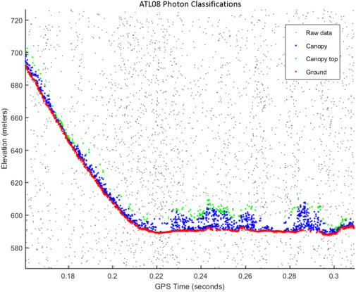
Fig. 4. An example of the classified photons produced from the ATL08 algorithm. Ground photons (red dots) are labeled as all photons falling within a point spread function distance of the estimated ground surface. The top of canopy photons (green dots) are photons that fall within a buffer distance from the upper canopy surface, and the photons that lie between the top of canopy surface and ground surface are labeled as canopy photons (blue dots). (Neuenschwander & Pitts, 2019)

Providing all the potentially useful information from all these processing steps results in a data file that looks like:

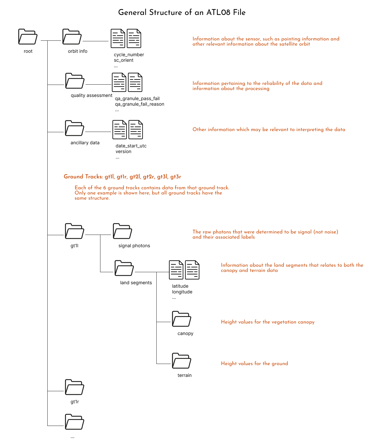
Another way to visualize these structure is to download one file and open it using https://myhdf5.hdfgroup.org/.

Further information about each one of the variables is available in the Algorithm Theoretical Basis Document (ATBD) for ATL08.

There is lots to explore in these variables, but we will move forward using a common ATL08 variable: h_canopy, or the “98% height of all the individual relative canopy heights (height above terrain)” (ATBD definition).

reader.vars.append(var_list=['h_canopy', 'latitude', 'longitude'])

Note that adding variables is a required step before you can load the data.

Load the data!

ds = reader.load()
ds

/srv/conda/envs/notebook/lib/python3.10/site-packages/icepyx/core/read.py:520: UserWarning: rename 'delta_time' to 'photon_idx' does not create an index anymore. Try using swap_dims instead or use set_index after rename to create an indexed coordinate.
  .rename({"delta_time": "photon_idx"})
/srv/conda/envs/notebook/lib/python3.10/site-packages/icepyx/core/read.py:520: UserWarning: rename 'delta_time' to 'photon_idx' does not create an index anymore. Try using swap_dims instead or use set_index after rename to create an indexed coordinate.
  .rename({"delta_time": "photon_idx"})

<xarray.Dataset>
Dimensions:              (gran_idx: 1, photon_idx: 211, spot: 2)
Coordinates:
  * gran_idx             (gran_idx) float64 5.54e+04
  * photon_idx           (photon_idx) int64 0 1 2 3 4 5 ... 206 207 208 209 210
  * spot                 (spot) uint8 1 2
    source_file          (gran_idx) <U74 './bosque_primavera_ATL08/processed_...
    delta_time           (photon_idx) datetime64[ns] 2019-05-04T12:47:13.5766...
Data variables:
    sc_orient            (gran_idx) int8 0
    cycle_number         (gran_idx) int8 3
    rgt                  (gran_idx, spot, photon_idx) float32 554.0 ... 554.0
    atlas_sdp_gps_epoch  (gran_idx) datetime64[ns] 2018-01-01T00:00:18
    data_start_utc       (gran_idx) datetime64[ns] 2019-05-04T12:46:31.876322
    data_end_utc         (gran_idx) datetime64[ns] 2019-05-04T12:48:54.200826
    latitude             (spot, gran_idx, photon_idx) float32 20.59 ... 20.73
    longitude            (spot, gran_idx, photon_idx) float32 -103.7 ... -103.7
    gt                   (gran_idx, spot) object 'gt3l' 'gt3r'
    h_canopy             (photon_idx) float32 12.12 4.747 11.83 ... nan nan nan
Attributes:
    data_product:  ATL08
    Description:   Contains data categorized as land at 100 meter intervals.
    data_rate:     Data are stored as aggregates of 100 meters.

xarray.Dataset

• Dimensions:
  • gran_idx: 1
  • photon_idx: 211
  • spot: 2
• Coordinates: (5)
  • gran_idx
    (gran_idx)
    float64
    5.54e+04

    array([55402.])

  • photon_idx
    (photon_idx)
    int64
    0 1 2 3 4 5 ... 206 207 208 209 210

    array([  0,   1,   2, ..., 208, 209, 210])

  • spot
    (spot)
    uint8
    1 2

    array([1, 2], dtype=uint8)

  • source_file
    (gran_idx)
    <U74
    './bosque_primavera_ATL08/proces...

    array(['./bosque_primavera_ATL08/processed_ATL08_20190504124152_05540301_006_02.h5'],
          dtype='<U74')

  • delta_time
    (photon_idx)
    datetime64[ns]
    2019-05-04T12:47:13.576668792 .....

    array(['2019-05-04T12:47:13.576668792', '2019-05-04T12:47:13.590795176',
           '2019-05-04T12:47:13.604878696', '2019-05-04T12:47:13.618858776',
           '2019-05-04T12:47:13.647116752', '2019-05-04T12:47:13.731658440',
           '2019-05-04T12:47:13.788115696', '2019-05-04T12:47:13.802188288',
           '2019-05-04T12:47:14.013615136', '2019-05-04T12:47:14.027716720',
           '2019-05-04T12:47:14.041828320', '2019-05-04T12:47:14.069985944',
           '2019-05-04T12:47:14.084116656', '2019-05-04T12:47:14.098204416',
           '2019-05-04T12:47:14.112308544', '2019-05-04T12:47:14.126439192',
           '2019-05-04T12:47:14.140474800', '2019-05-04T12:47:14.154503088',
           '2019-05-04T12:47:14.168615944', '2019-05-04T12:47:14.182727944',
           '2019-05-04T12:47:14.196803520', '2019-05-04T12:47:14.225002096',
           '2019-05-04T12:47:14.239145008', '2019-05-04T12:47:14.253240544',
           '2019-05-04T12:47:14.267282136', '2019-05-04T12:47:14.281345400',
           '2019-05-04T12:47:14.295463616', '2019-05-04T12:47:14.309582960',
           '2019-05-04T12:47:14.323643288', '2019-05-04T12:47:14.337699200',
           '2019-05-04T12:47:14.351769576', '2019-05-04T12:47:14.363045864',
           '2019-05-04T12:47:14.379987728', '2019-05-04T12:47:14.394098040',
           '2019-05-04T12:47:14.408184296', '2019-05-04T12:47:14.422336984',
           '2019-05-04T12:47:14.436399800', '2019-05-04T12:47:14.450439312',
           '2019-05-04T12:47:14.464605056', '2019-05-04T12:47:14.478736368',
    ...
           '2019-05-04T12:47:15.425911016', '2019-05-04T12:47:15.439995088',
           '2019-05-04T12:47:15.454061472', '2019-05-04T12:47:15.468143592',
           '2019-05-04T12:47:15.482238848', '2019-05-04T12:47:15.496324880',
           '2019-05-04T12:47:15.510409496', '2019-05-04T12:47:15.524510280',
           '2019-05-04T12:47:15.538615648', '2019-05-04T12:47:15.566816696',
           '2019-05-04T12:47:15.580919696', '2019-05-04T12:47:15.594985688',
           '2019-05-04T12:47:15.609048944', '2019-05-04T12:47:15.623173096',
           '2019-05-04T12:47:15.637281512', '2019-05-04T12:47:15.651381832',
           '2019-05-04T12:47:15.665494736', '2019-05-04T12:47:15.679564576',
           '2019-05-04T12:47:15.693640304', '2019-05-04T12:47:15.707745176',
           '2019-05-04T12:47:15.721833264', '2019-05-04T12:47:15.735931400',
           '2019-05-04T12:47:15.750026272', '2019-05-04T12:47:15.764102288',
           '2019-05-04T12:47:15.778227184', '2019-05-04T12:47:15.806428968',
           '2019-05-04T12:47:15.820523432', '2019-05-04T12:47:15.834607024',
           '2019-05-04T12:47:15.848673504', '2019-05-04T12:47:15.862757488',
           '2019-05-04T12:47:15.876856944', '2019-05-04T12:47:15.890974768',
           '2019-05-04T12:47:15.905085432', '2019-05-04T12:47:15.919119064',
           '2019-05-04T12:47:15.933193432', '2019-05-04T12:47:15.947348696',
           '2019-05-04T12:47:15.961461904', '2019-05-04T12:47:15.975561616',
           '2019-05-04T12:47:15.989663088'], dtype='datetime64[ns]')

• Data variables: (10)
  • sc_orient
    (gran_idx)
    int8
    0

    array([0], dtype=int8)

  • cycle_number
    (gran_idx)
    int8
    3

    array([3], dtype=int8)

  • rgt
    (gran_idx, spot, photon_idx)
    float32
    554.0 554.0 554.0 ... 554.0 554.0

    contentType :

    referenceInformation

    description :

    The reference ground track (RGT) is the track on the earth at which a specified unit vector within the observatory is pointed. Under nominal operating conditions, there will be no data collected along the RGT, as the RGT is spanned by GT3 and GT4. During slews or off-pointing, it is possible that ground tracks may intersect the RGT. The ICESat-2 mission has 1387 RGTs.

    long_name :

    reference ground track

    source :

    Operations

    units :

    1

    valid_max :

    1387

    valid_min :

    1

    array([[[554., 554., 554., 554., 554., 554., 554., 554., 554., 554.,
             554., 554., 554., 554., 554., 554., 554., 554., 554., 554.,
             554., 554., 554., 554., 554., 554., 554., 554., 554., 554.,
             554., 554., 554., 554., 554., 554., 554., 554., 554., 554.,
             554., 554., 554., 554., 554., 554., 554., 554., 554., 554.,
             554., 554., 554., 554., 554., 554., 554., 554., 554., 554.,
             554., 554., 554., 554., 554., 554., 554., 554., 554., 554.,
             554., 554., 554., 554., 554., 554., 554., 554., 554., 554.,
             554., 554., 554., 554., 554., 554., 554., 554., 554., 554.,
             554., 554., 554., 554., 554., 554., 554., 554., 554., 554.,
             554., 554., 554., 554., 554., 554., 554., 554., 554., 554.,
             554., 554., 554., 554., 554., 554., 554., 554., 554., 554.,
              nan,  nan,  nan,  nan,  nan,  nan,  nan,  nan,  nan,  nan,
              nan,  nan,  nan,  nan,  nan,  nan,  nan,  nan,  nan,  nan,
              nan,  nan,  nan,  nan,  nan,  nan,  nan,  nan,  nan,  nan,
              nan,  nan,  nan,  nan,  nan,  nan,  nan,  nan,  nan,  nan,
              nan,  nan,  nan,  nan,  nan,  nan,  nan,  nan,  nan,  nan,
              nan,  nan,  nan,  nan,  nan,  nan,  nan,  nan,  nan,  nan,
              nan,  nan,  nan,  nan,  nan,  nan,  nan,  nan,  nan,  nan,
              nan,  nan,  nan,  nan,  nan,  nan,  nan,  nan,  nan,  nan,
    ...
              nan,  nan,  nan,  nan,  nan,  nan,  nan,  nan,  nan,  nan,
              nan,  nan,  nan,  nan,  nan,  nan,  nan,  nan,  nan,  nan,
              nan,  nan,  nan,  nan,  nan,  nan,  nan,  nan,  nan,  nan,
              nan,  nan,  nan,  nan,  nan,  nan,  nan,  nan,  nan,  nan,
              nan,  nan,  nan,  nan,  nan,  nan,  nan,  nan,  nan,  nan,
              nan,  nan,  nan,  nan,  nan,  nan,  nan,  nan,  nan,  nan,
              nan,  nan,  nan,  nan,  nan,  nan,  nan,  nan,  nan,  nan,
              nan,  nan,  nan,  nan,  nan,  nan,  nan,  nan,  nan,  nan,
              nan,  nan,  nan,  nan,  nan,  nan,  nan,  nan,  nan,  nan,
              nan,  nan,  nan,  nan,  nan,  nan,  nan,  nan,  nan,  nan,
             554., 554., 554., 554., 554., 554., 554., 554., 554., 554.,
             554., 554., 554., 554., 554., 554., 554., 554., 554., 554.,
             554., 554., 554., 554., 554., 554., 554., 554., 554., 554.,
             554., 554., 554., 554., 554., 554., 554., 554., 554., 554.,
             554., 554., 554., 554., 554., 554., 554., 554., 554., 554.,
             554., 554., 554., 554., 554., 554., 554., 554., 554., 554.,
             554., 554., 554., 554., 554., 554., 554., 554., 554., 554.,
             554., 554., 554., 554., 554., 554., 554., 554., 554., 554.,
             554., 554., 554., 554., 554., 554., 554., 554., 554., 554.,
             554.]]], dtype=float32)

  • atlas_sdp_gps_epoch
    (gran_idx)
    datetime64[ns]
    2018-01-01T00:00:18

    array(['2018-01-01T00:00:18.000000000'], dtype='datetime64[ns]')

  • data_start_utc
    (gran_idx)
    datetime64[ns]
    2019-05-04T12:46:31.876322

    array(['2019-05-04T12:46:31.876322000'], dtype='datetime64[ns]')

  • data_end_utc
    (gran_idx)
    datetime64[ns]
    2019-05-04T12:48:54.200826

    array(['2019-05-04T12:48:54.200826000'], dtype='datetime64[ns]')

  • latitude
    (spot, gran_idx, photon_idx)
    float32
    20.59 20.59 20.59 ... 20.72 20.73

    contentType :

    modelResult

    description :

    Latitude of the center-most signal photon within each segment.

    long_name :

    latitude

    source :

    Land ATBD section 2.4

    standard_name :

    latitude

    units :

    degrees

    valid_max :

    90.0

    valid_min :

    -90.0

    array([[[20.592943, 20.593845, 20.594746, 20.595648, 20.59745 ,
             20.60286 , 20.606464, 20.607367, 20.620888, 20.621788,
             20.62269 , 20.624493, 20.625395, 20.626297, 20.627197,
             20.6281  , 20.629   , 20.629902, 20.630804, 20.631704,
             20.632607, 20.634409, 20.635311, 20.636211, 20.637114,
             20.638014, 20.638916, 20.639816, 20.640718, 20.64162 ,
             20.642523, 20.643244, 20.644325, 20.645226, 20.646128,
             20.64703 , 20.64793 , 20.648832, 20.649734, 20.650635,
             20.651537, 20.652437, 20.65334 , 20.65424 , 20.655142,
             20.656044, 20.656944, 20.657846, 20.658749, 20.659649,
             20.660551, 20.661451, 20.662354, 20.663254, 20.664156,
             20.665058, 20.665958, 20.66686 , 20.667763, 20.668663,
             20.669565, 20.670467, 20.671368, 20.67227 , 20.67317 ,
             20.674072, 20.674973, 20.675875, 20.676777, 20.677677,
             20.67858 , 20.679482, 20.680382, 20.681284, 20.682184,
             20.683086, 20.683989, 20.684889, 20.685791, 20.686691,
             20.687593, 20.688496, 20.689217, 20.690298, 20.691198,
             20.6921  , 20.693003, 20.693903, 20.694805, 20.695707,
             20.696608, 20.69751 , 20.69841 , 20.699312, 20.700212,
             20.701115, 20.702017, 20.702917, 20.70382 , 20.704721,
    ...
                   nan,       nan,       nan,       nan,       nan,
             20.625654, 20.626554, 20.627457, 20.628359, 20.635569,
             20.63647 , 20.637373, 20.638273, 20.639175, 20.640078,
             20.640978, 20.644585, 20.646387, 20.647287, 20.64819 ,
             20.649992, 20.650894, 20.651796, 20.652697, 20.653599,
             20.655401, 20.656303, 20.657204, 20.658106, 20.659006,
             20.659908, 20.662613, 20.663513, 20.664415, 20.666218,
             20.66712 , 20.66802 , 20.668922, 20.669825, 20.670725,
             20.671627, 20.672527, 20.67343 , 20.674332, 20.675232,
             20.676134, 20.677036, 20.677937, 20.678839, 20.679739,
             20.680641, 20.681543, 20.682444, 20.68605 , 20.68695 ,
             20.687853, 20.688753, 20.689655, 20.690557, 20.691458,
             20.69236 , 20.693262, 20.694162, 20.695065, 20.695965,
             20.696867, 20.69867 , 20.699572, 20.700472, 20.701374,
             20.702274, 20.703176, 20.704079, 20.704979, 20.705881,
             20.706781, 20.707684, 20.708586, 20.709486, 20.710388,
             20.711288, 20.71219 , 20.713993, 20.714895, 20.715796,
             20.716698, 20.7176  , 20.7185  , 20.719402, 20.720304,
             20.721205, 20.722107, 20.723007, 20.72391 , 20.724812,
             20.725712]]], dtype=float32)

  • longitude
    (spot, gran_idx, photon_idx)
    float32
    -103.7 -103.7 ... -103.7 -103.7

    contentType :

    modelResult

    description :

    Longitude of the center-most signal photon within each segment.

    long_name :

    longitude

    source :

    Land ATBD section 2.4

    standard_name :

    longitude

    units :

    degrees

    valid_max :

    180.0

    valid_min :

    -180.0

    array([[[-103.67242 , -103.672516, -103.67261 , -103.6727  ,
             -103.6729  , -103.67346 , -103.673836, -103.673935,
             -103.67535 , -103.675446, -103.67554 , -103.67573 ,
             -103.67583 , -103.67592 , -103.67601 , -103.67611 ,
             -103.6762  , -103.6763  , -103.67639 , -103.67649 ,
             -103.67658 , -103.676765, -103.676865, -103.676956,
             -103.67705 , -103.67715 , -103.677246, -103.677345,
             -103.67743 , -103.67753 , -103.67762 , -103.6777  ,
             -103.67781 , -103.67791 , -103.678   , -103.678085,
             -103.678185, -103.67828 , -103.678375, -103.678474,
             -103.678566, -103.67866 , -103.67876 , -103.678856,
             -103.67895 , -103.67904 , -103.67913 , -103.67922 ,
             -103.67932 , -103.67941 , -103.679504, -103.6796  ,
             -103.6797  , -103.6798  , -103.67989 , -103.679985,
             -103.68008 , -103.680176, -103.68027 , -103.68037 ,
             -103.68046 , -103.68055 , -103.68064 , -103.68073 ,
             -103.68083 , -103.68093 , -103.68103 , -103.68112 ,
             -103.68121 , -103.681305, -103.6814  , -103.68149 ,
             -103.68159 , -103.68169 , -103.681786, -103.68188 ,
             -103.68197 , -103.68207 , -103.68216 , -103.68226 ,
    ...
             -103.67717 , -103.67727 , -103.67736 , -103.67754 ,
             -103.67764 , -103.677734, -103.67783 , -103.677925,
             -103.678116, -103.67821 , -103.67831 , -103.6784  ,
             -103.6785  , -103.67859 , -103.67887 , -103.67897 ,
             -103.67906 , -103.67925 , -103.679344, -103.67944 ,
             -103.679535, -103.67963 , -103.67972 , -103.67982 ,
             -103.67991 , -103.68001 , -103.6801  , -103.68019 ,
             -103.68029 , -103.68038 , -103.68047 , -103.68057 ,
             -103.68067 , -103.68076 , -103.680855, -103.680954,
             -103.68133 , -103.68143 , -103.68152 , -103.68161 ,
             -103.68171 , -103.6818  , -103.68189 , -103.681984,
             -103.68208 , -103.68218 , -103.682274, -103.682365,
             -103.682465, -103.682655, -103.682755, -103.682846,
             -103.68294 , -103.68304 , -103.68313 , -103.68322 ,
             -103.68332 , -103.68341 , -103.68351 , -103.6836  ,
             -103.68369 , -103.68379 , -103.68388 , -103.68398 ,
             -103.684074, -103.684265, -103.68436 , -103.684456,
             -103.68455 , -103.68465 , -103.68474 , -103.68483 ,
             -103.68493 , -103.68502 , -103.68511 , -103.68521 ,
             -103.6853  , -103.6854  , -103.68549 ]]], dtype=float32)

  • gt
    (gran_idx, spot)
    object
    'gt3l' 'gt3r'

    array([['gt3l', 'gt3r']], dtype=object)

  • h_canopy
    (photon_idx)
    float32
    12.12 4.747 11.83 ... nan nan nan

    contentType :

    modelResult

    coordinates :

    ../delta_time ../latitude ../longitude

    description :

    98% height of all the individual canopy relative heights for the segment above the estimated terrain surface. Relative canopy heights have been computed by differencing the canopy photon height from the estimated terrain surface.

    long_name :

    height canopy

    source :

    Land ATBD section 4.12

    units :

    meters

    array([12.117554 ,  4.7471924, 11.826294 , 12.599121 ,        nan,
           18.487427 ,        nan, 24.531128 , 23.573975 ,  6.973877 ,
           15.614014 , 18.686768 , 10.208862 , 19.486816 , 19.792969 ,
           24.182617 , 26.141113 ,        nan, 27.215698 , 27.964355 ,
           28.768066 , 23.500977 , 20.939087 , 12.468384 , 12.3302   ,
           12.56543  , 18.28833  ,        nan,  3.2608643, 15.973389 ,
           20.57251  , 16.383667 , 19.53479  , 19.167236 ,  8.956299 ,
           10.339844 ,  6.9119873,        nan,  6.6381836, 13.006592 ,
           10.125366 ,  7.1741943,  6.220581 , 13.171265 , 13.741211 ,
           14.266846 , 13.998291 ,  6.2819824, 10.767212 ,        nan,
           11.753906 , 19.83789  ,  8.949463 ,  6.9605713, 17.22107  ,
           20.040527 ,  8.8289795, 10.093262 ,  6.963379 , 10.654053 ,
           13.63623  ,  8.8897705,        nan,  8.487671 ,  4.117676 ,
            2.7399902,  5.741211 ,  9.786987 ,  5.447876 ,  6.3466797,
            2.6264648,        nan,        nan, 14.463623 , 19.986572 ,
           26.920166 , 23.636475 , 20.366577 , 23.44165  , 18.091675 ,
           12.490723 , 21.749268 , 10.508667 , 18.734863 , 16.601318 ,
            7.385254 ,        nan,        nan,  9.800293 ,  5.3067627,
           12.211426 , 15.874878 ,  8.875732 , 15.800903 , 12.877563 ,
                  nan,        nan,  2.3807373,  6.1132812,        nan,
    ...
                  nan,  5.647461 ,  8.42688  ,        nan,        nan,
           28.482422 , 41.51538  , 36.190186 , 44.303833 , 54.733765 ,
           48.05542  , 30.716309 ,        nan, 23.340576 , 38.804565 ,
           44.656982 , 30.472778 , 22.952637 , 12.519897 , 16.93335  ,
           30.526001 , 30.635742 , 20.736328 , 29.40503  , 11.497925 ,
           20.793457 , 15.886963 , 18.502075 , 12.783813 ,        nan,
                  nan, 16.045044 , 12.643677 , 13.928345 , 10.867432 ,
            9.350586 ,  8.6102295, 20.031738 , 20.65039  ,  9.560913 ,
           14.163574 , 16.621704 ,        nan,        nan,        nan,
           10.887817 , 12.17334  , 11.110474 , 11.06665  , 10.12915  ,
           11.172485 , 10.751099 ,  3.20813  , 16.136719 , 16.071533 ,
           16.224487 , 18.876953 , 30.146606 , 22.111328 ,        nan,
                  nan,        nan,        nan, 12.220581 , 14.92688  ,
                  nan, 13.107788 ,  7.1689453,  7.2957764,        nan,
                  nan,        nan,        nan,        nan,  9.05249  ,
                  nan,        nan,        nan,        nan,        nan,
                  nan,        nan,        nan,        nan,        nan,
                  nan,        nan,        nan,        nan,        nan,
                  nan,        nan,        nan,        nan,        nan,
                  nan], dtype=float32)

• Indexes: (3)
  • gran_idx
    PandasIndex

    PandasIndex(Float64Index([55402.0], dtype='float64', name='gran_idx'))

  • photon_idx
    PandasIndex

    PandasIndex(Int64Index([  0,   1,   2,   3,   4,   5,   6,   7,   8,   9,
                ...
                201, 202, 203, 204, 205, 206, 207, 208, 209, 210],
               dtype='int64', name='photon_idx', length=211))

  • spot
    PandasIndex

    PandasIndex(UInt64Index([1, 2], dtype='uint64', name='spot'))

• Attributes: (3)

  data_product :

  ATL08

  Description :

  Contains data categorized as land at 100 meter intervals.

  data_rate :

  Data are stored as aggregates of 100 meters.

Here we have an xarray Dataset, a common Python data structure for analysis. To visualize the data we can plot it using:

ds.plot.scatter(x="longitude", y="latitude", hue="h_canopy")

<matplotlib.collections.PathCollection at 0x7f3d005d8430>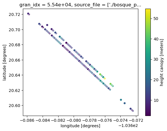

Notice also that the data is shown for just our area of interest! That is because of icepyx’s subsetting feature, which we will discuss more in the next section.

Using icepyx to download a subset of a granule

One feature which is not yet available in earthaccess is the ability to download just a subset of the file. This could mean a smaller spatial area or fewer variables. This feature is available in icepyx.

We saw above that icepyx by default will subset your data to the bounding box you provided when downloading. If you know in advance which variables you want icepyx can also subset variables.

Subset variables

# Create our Query
short_name = 'ATL08'
spatial_extent = list(bosque.bounds)
date_range = ['2019-05-04','2019-05-04']
region = ipx.Query(short_name, spatial_extent, date_range)

# Specify desired variables
region.order_vars.append(var_list=['h_canopy', 'latitude', 'longitude'])

We are already authenticated with NASA EDL

# Download the granules, using the Coverage kwarg to specify variables
region.download_granules(path='./ATL08_h_canopy', Coverage=region.order_vars.wanted)

Total number of data order requests is  1  for  1  granules.
Data request  1  of  1  is submitting to NSIDC
order ID:  5000004610386
Initial status of your order request at NSIDC is:  processing
Your order status is still  processing  at NSIDC. Please continue waiting... this may take a few moments.
Your order is: complete
Beginning download of zipped output...
Data request 5000004610386 of  1  order(s) is downloaded.
Download complete

# Read the new data
pattern = "processed_ATL{product:2}_{datetime:%Y%m%d%H%M%S}_{rgt:4}{cycle:2}{orbitsegment:2}_{version:3}_{revision:2}.h5"
reader = ipx.Read('./ATL08_h_canopy', "ATL08", pattern)

You have 1 files matching the filename pattern to be read in.

The available variables list on the subset dataset is a lot shorter!

reader.vars.avail()

['ancillary_data/atlas_sdp_gps_epoch',
 'ancillary_data/data_end_utc',
 'ancillary_data/data_start_utc',
 'ancillary_data/end_delta_time',
 'ancillary_data/granule_end_utc',
 'ancillary_data/granule_start_utc',
 'ancillary_data/start_delta_time',
 'gt3l/land_segments/canopy/h_canopy',
 'gt3l/land_segments/delta_time',
 'gt3l/land_segments/latitude',
 'gt3l/land_segments/longitude',
 'gt3r/land_segments/canopy/h_canopy',
 'gt3r/land_segments/delta_time',
 'gt3r/land_segments/latitude',
 'gt3r/land_segments/longitude',
 'orbit_info/sc_orient',
 'orbit_info/sc_orient_time']

Some example plots

To close, here are a few more examples of reading and visualizing ATL08 data.

Example 1: View the photon classifications

# Set up the data reader
pattern = "processed_ATL{product:2}_{datetime:%Y%m%d%H%M%S}_{rgt:4}{cycle:2}{orbitsegment:2}_{version:3}_{revision:2}.h5"
reader = ipx.Read('./bosque_primavera_ATL08', "ATL08", pattern)

You have 1 files matching the filename pattern to be read in.

# Add the photon height and classification variables
reader.vars.append(var_list=['ph_h', 'classed_pc_flag', 'latitude', 'longitude'])

# load the dataset
ds_photons = reader.load()
ds_photons

/srv/conda/envs/notebook/lib/python3.10/site-packages/icepyx/core/read.py:520: UserWarning: rename 'delta_time' to 'photon_idx' does not create an index anymore. Try using swap_dims instead or use set_index after rename to create an indexed coordinate.
  .rename({"delta_time": "photon_idx"})
/srv/conda/envs/notebook/lib/python3.10/site-packages/icepyx/core/read.py:520: UserWarning: rename 'delta_time' to 'photon_idx' does not create an index anymore. Try using swap_dims instead or use set_index after rename to create an indexed coordinate.
  .rename({"delta_time": "photon_idx"})
/srv/conda/envs/notebook/lib/python3.10/site-packages/icepyx/core/read.py:520: UserWarning: rename 'delta_time' to 'photon_idx' does not create an index anymore. Try using swap_dims instead or use set_index after rename to create an indexed coordinate.
  .rename({"delta_time": "photon_idx"})
/srv/conda/envs/notebook/lib/python3.10/site-packages/icepyx/core/read.py:520: UserWarning: rename 'delta_time' to 'photon_idx' does not create an index anymore. Try using swap_dims instead or use set_index after rename to create an indexed coordinate.
  .rename({"delta_time": "photon_idx"})

<xarray.Dataset>
Dimensions:              (gran_idx: 1, photon_idx: 25234, spot: 2)
Coordinates:
  * gran_idx             (gran_idx) float64 5.54e+04
  * photon_idx           (photon_idx) int64 0 1 2 3 ... 25230 25231 25232 25233
  * spot                 (spot) uint8 1 2
    source_file          (gran_idx) <U74 './bosque_primavera_ATL08/processed_...
    delta_time           (photon_idx) datetime64[ns] 2019-05-04T12:47:13.5766...
Data variables:
    sc_orient            (gran_idx) int8 0
    cycle_number         (gran_idx) int8 3
    rgt                  (gran_idx, spot, photon_idx) float32 554.0 ... nan
    atlas_sdp_gps_epoch  (gran_idx) datetime64[ns] 2018-01-01T00:00:18
    data_start_utc       (gran_idx) datetime64[ns] 2019-05-04T12:46:31.876322
    data_end_utc         (gran_idx) datetime64[ns] 2019-05-04T12:48:54.200826
    latitude             (spot, gran_idx, photon_idx) float32 20.59 ... nan
    longitude            (spot, gran_idx, photon_idx) float32 -103.7 ... nan
    gt                   (gran_idx, spot) <U4 'gt3l' 'gt3r'
    ph_h                 (spot, gran_idx, photon_idx) float32 nan ... 0.05542
    classed_pc_flag      (spot, gran_idx, photon_idx) float32 nan nan ... 1.0
Attributes:
    data_product:  ATL08

xarray.Dataset

• Dimensions:
  • gran_idx: 1
  • photon_idx: 25234
  • spot: 2
• Coordinates: (5)
  • gran_idx
    (gran_idx)
    float64
    5.54e+04

    array([55402.])

  • photon_idx
    (photon_idx)
    int64
    0 1 2 3 ... 25230 25231 25232 25233

    array([    0,     1,     2, ..., 25231, 25232, 25233])

  • spot
    (spot)
    uint8
    1 2

    array([1, 2], dtype=uint8)

  • source_file
    (gran_idx)
    <U74
    './bosque_primavera_ATL08/proces...

    array(['./bosque_primavera_ATL08/processed_ATL08_20190504124152_05540301_006_02.h5'],
          dtype='<U74')

  • delta_time
    (photon_idx)
    datetime64[ns]
    2019-05-04T12:47:13.576668792 .....

    array(['2019-05-04T12:47:13.576668792', '2019-05-04T12:47:13.590795176',
           '2019-05-04T12:47:13.604878696', ...,
           '2019-05-04T12:47:15.995923304', '2019-05-04T12:47:15.996123296',
           '2019-05-04T12:47:15.996323304'], dtype='datetime64[ns]')

• Data variables: (11)
  • sc_orient
    (gran_idx)
    int8
    0

    array([0], dtype=int8)

  • cycle_number
    (gran_idx)
    int8
    3

    array([3], dtype=int8)

  • rgt
    (gran_idx, spot, photon_idx)
    float32
    554.0 554.0 554.0 ... nan nan nan

    contentType :

    referenceInformation

    description :

    The reference ground track (RGT) is the track on the earth at which a specified unit vector within the observatory is pointed. Under nominal operating conditions, there will be no data collected along the RGT, as the RGT is spanned by GT3 and GT4. During slews or off-pointing, it is possible that ground tracks may intersect the RGT. The ICESat-2 mission has 1387 RGTs.

    long_name :

    reference ground track

    source :

    Operations

    units :

    1

    valid_max :

    1387

    valid_min :

    1

    array([[[554., 554., 554., ...,  nan,  nan,  nan],
            [ nan,  nan,  nan, ...,  nan,  nan,  nan]]], dtype=float32)

  • atlas_sdp_gps_epoch
    (gran_idx)
    datetime64[ns]
    2018-01-01T00:00:18

    array(['2018-01-01T00:00:18.000000000'], dtype='datetime64[ns]')

  • data_start_utc
    (gran_idx)
    datetime64[ns]
    2019-05-04T12:46:31.876322

    array(['2019-05-04T12:46:31.876322000'], dtype='datetime64[ns]')

  • data_end_utc
    (gran_idx)
    datetime64[ns]
    2019-05-04T12:48:54.200826

    array(['2019-05-04T12:48:54.200826000'], dtype='datetime64[ns]')

  • latitude
    (spot, gran_idx, photon_idx)
    float32
    20.59 20.59 20.59 ... nan nan nan

    contentType :

    modelResult

    description :

    Latitude of the center-most signal photon within each segment.

    long_name :

    latitude

    source :

    Land ATBD section 2.4

    standard_name :

    latitude

    units :

    degrees

    valid_max :

    90.0

    valid_min :

    -90.0

    array([[[20.592943, 20.593845, 20.594746, ...,       nan,       nan,
                   nan]],
    
           [[      nan,       nan,       nan, ...,       nan,       nan,
                   nan]]], dtype=float32)

  • longitude
    (spot, gran_idx, photon_idx)
    float32
    -103.7 -103.7 -103.7 ... nan nan

    contentType :

    modelResult

    description :

    Longitude of the center-most signal photon within each segment.

    long_name :

    longitude

    source :

    Land ATBD section 2.4

    standard_name :

    longitude

    units :

    degrees

    valid_max :

    180.0

    valid_min :

    -180.0

    array([[[-103.67242 , -103.672516, -103.67261 , ...,         nan,
                     nan,         nan]],
    
           [[        nan,         nan,         nan, ...,         nan,
                     nan,         nan]]], dtype=float32)

  • gt
    (gran_idx, spot)
    <U4
    'gt3l' 'gt3r'

    array([['gt3l', 'gt3r']], dtype='<U4')

  • ph_h
    (spot, gran_idx, photon_idx)
    float32
    nan nan nan ... 0.05103 0.05542

    contentType :

    physicalMeasurement

    description :

    Height of photons above interpolated land surface

    long_name :

    relative photon height

    source :

    land/veg ATBD, 15May2020, Section 2.3.4

    standard_name :

    height

    units :

    meters

    array([[[       nan,        nan,        nan, ...,        nan,
                    nan,        nan]],
    
           [[       nan,        nan,        nan, ..., 0.15209961,
             0.05102539, 0.05541992]]], dtype=float32)

  • classed_pc_flag
    (spot, gran_idx, photon_idx)
    float32
    nan nan nan nan ... 1.0 1.0 1.0 1.0

    contentType :

    modelResult

    description :

    Land Vegetation ATBD classification flag for each photon as either noise, ground, canopy, and top of canopy. 0 = noise, 1 = ground, 2 = canopy, or 3 = top of canopy.

    flag_meanings :

    noise ground canopy top_of_canopy

    flag_values :

    [0 1 2 3]

    long_name :

    photon land atbd classification

    source :

    Land ATBD section 4.10

    units :

    1

    array([[[nan, nan, nan, ..., nan, nan, nan]],
    
           [[nan, nan, nan, ...,  1.,  1.,  1.]]], dtype=float32)

• Indexes: (3)
  • gran_idx
    PandasIndex

    PandasIndex(Float64Index([55402.0], dtype='float64', name='gran_idx'))

  • photon_idx
    PandasIndex

    PandasIndex(Int64Index([    0,     1,     2,     3,     4,     5,     6,     7,     8,
                    9,
                ...
                25224, 25225, 25226, 25227, 25228, 25229, 25230, 25231, 25232,
                25233],
               dtype='int64', name='photon_idx', length=25234))

  • spot
    PandasIndex

    PandasIndex(UInt64Index([1, 2], dtype='uint64', name='spot'))

• Attributes: (1)

  data_product :

  ATL08

# Select just one beam
gt1l = ds_photons.sel(spot=1)

# A less complex plot
fig, ax = plt.subplots()
fig.set_size_inches(15, 4)
    
gt1l.plot.scatter(ax=ax, x='delta_time', y='ph_h', hue='classed_pc_flag')

<matplotlib.collections.PathCollection at 0x7f3cfe539e10>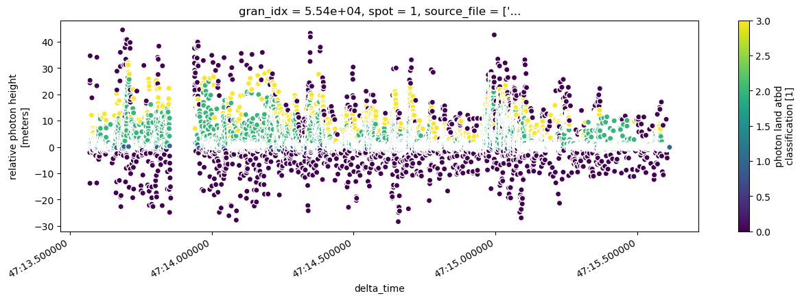

# A plot with more customization
fig, ax = plt.subplots()
fig.set_size_inches(17, 6)
fig.suptitle('Classification of input photons', size=16)

labels={0: 'noise', 1: 'ground', 2: 'canopy', 3: 'top of canopy'}
colors={0: 'grey', 1: 'red', 2: 'green', 3: 'blue'}

for g in np.unique(gt1l.classed_pc_flag[0]):
    if not math.isnan(g):
        ds_group = gt1l.where(gt1l.classed_pc_flag == g, drop=True)
        ax.scatter(x=ds_group.delta_time, y=ds_group.ph_h, c=colors[g], 
                   label=labels[g], s=8)
ax.legend()

ax.set_ylabel('Height above the ground (m)', size=12)

Text(0, 0.5, 'Height above the ground (m)')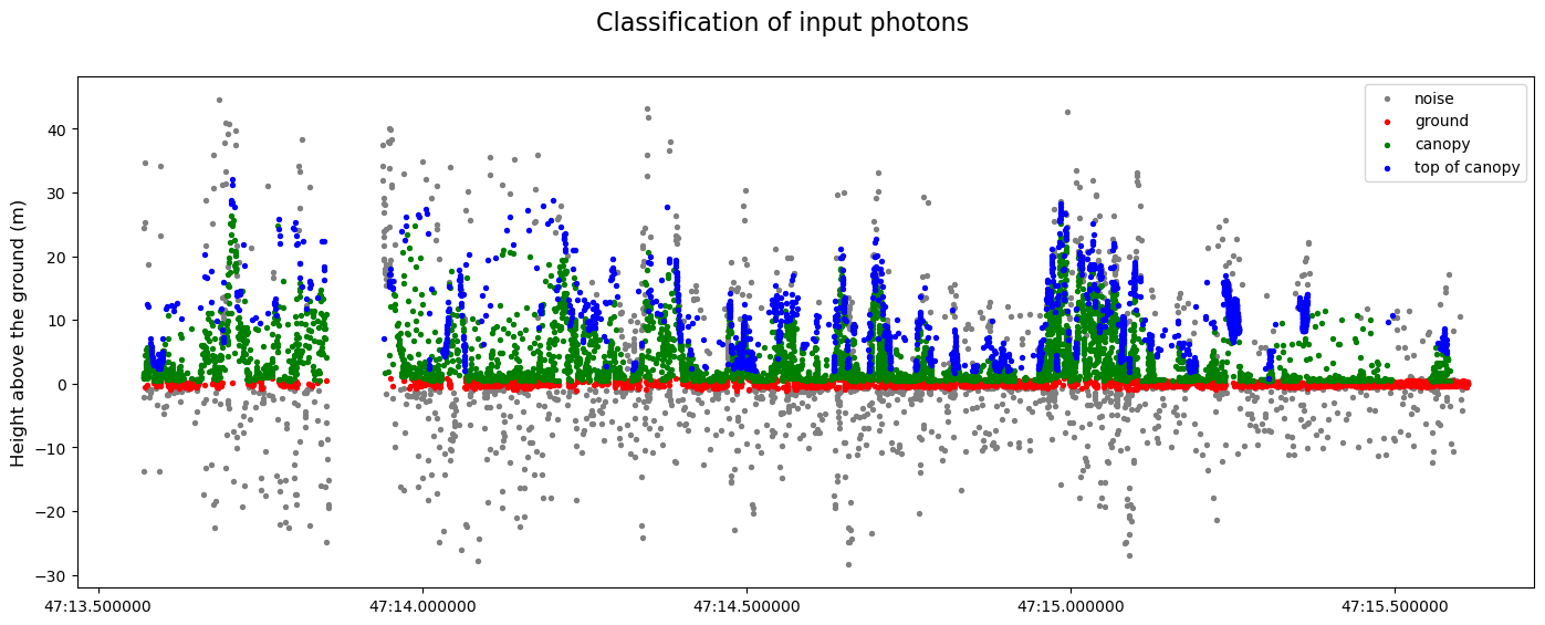

Plot the canopy compared to the ground height

# Remove our previous variables
reader.vars.remove(all=True)
# Add the next set of variables to the list
reader.vars.append(var_list=['h_te_best_fit', 'latitude', 'longitude'])

# load the data
ds_te = reader.load()
ds_te

/srv/conda/envs/notebook/lib/python3.10/site-packages/icepyx/core/read.py:520: UserWarning: rename 'delta_time' to 'photon_idx' does not create an index anymore. Try using swap_dims instead or use set_index after rename to create an indexed coordinate.
  .rename({"delta_time": "photon_idx"})
/srv/conda/envs/notebook/lib/python3.10/site-packages/icepyx/core/read.py:520: UserWarning: rename 'delta_time' to 'photon_idx' does not create an index anymore. Try using swap_dims instead or use set_index after rename to create an indexed coordinate.
  .rename({"delta_time": "photon_idx"})

<xarray.Dataset>
Dimensions:              (gran_idx: 1, photon_idx: 211, spot: 2)
Coordinates:
  * gran_idx             (gran_idx) float64 5.54e+04
  * photon_idx           (photon_idx) int64 0 1 2 3 4 5 ... 206 207 208 209 210
  * spot                 (spot) uint8 1 2
    source_file          (gran_idx) <U74 './bosque_primavera_ATL08/processed_...
    delta_time           (photon_idx) datetime64[ns] 2019-05-04T12:47:13.5766...
Data variables:
    sc_orient            (gran_idx) int8 0
    cycle_number         (gran_idx) int8 3
    rgt                  (gran_idx, spot, photon_idx) float32 554.0 ... 554.0
    atlas_sdp_gps_epoch  (gran_idx) datetime64[ns] 2018-01-01T00:00:18
    data_start_utc       (gran_idx) datetime64[ns] 2019-05-04T12:46:31.876322
    data_end_utc         (gran_idx) datetime64[ns] 2019-05-04T12:48:54.200826
    latitude             (spot, gran_idx, photon_idx) float32 20.59 ... 20.73
    longitude            (spot, gran_idx, photon_idx) float32 -103.7 ... -103.7
    gt                   (gran_idx, spot) object 'gt3l' 'gt3r'
    h_te_best_fit        (photon_idx) float32 1.342e+03 1.34e+03 ... 1.381e+03
Attributes:
    data_product:  ATL08
    Description:   Contains data categorized as land at 100 meter intervals.
    data_rate:     Data are stored as aggregates of 100 meters.

xarray.Dataset

• Dimensions:
  • gran_idx: 1
  • photon_idx: 211
  • spot: 2
• Coordinates: (5)
  • gran_idx
    (gran_idx)
    float64
    5.54e+04

    array([55402.])

  • photon_idx
    (photon_idx)
    int64
    0 1 2 3 4 5 ... 206 207 208 209 210

    array([  0,   1,   2, ..., 208, 209, 210])

  • spot
    (spot)
    uint8
    1 2

    array([1, 2], dtype=uint8)

  • source_file
    (gran_idx)
    <U74
    './bosque_primavera_ATL08/proces...

    array(['./bosque_primavera_ATL08/processed_ATL08_20190504124152_05540301_006_02.h5'],
          dtype='<U74')

  • delta_time
    (photon_idx)
    datetime64[ns]
    2019-05-04T12:47:13.576668792 .....

    array(['2019-05-04T12:47:13.576668792', '2019-05-04T12:47:13.590795176',
           '2019-05-04T12:47:13.604878696', '2019-05-04T12:47:13.618858776',
           '2019-05-04T12:47:13.647116752', '2019-05-04T12:47:13.731658440',
           '2019-05-04T12:47:13.788115696', '2019-05-04T12:47:13.802188288',
           '2019-05-04T12:47:14.013615136', '2019-05-04T12:47:14.027716720',
           '2019-05-04T12:47:14.041828320', '2019-05-04T12:47:14.069985944',
           '2019-05-04T12:47:14.084116656', '2019-05-04T12:47:14.098204416',
           '2019-05-04T12:47:14.112308544', '2019-05-04T12:47:14.126439192',
           '2019-05-04T12:47:14.140474800', '2019-05-04T12:47:14.154503088',
           '2019-05-04T12:47:14.168615944', '2019-05-04T12:47:14.182727944',
           '2019-05-04T12:47:14.196803520', '2019-05-04T12:47:14.225002096',
           '2019-05-04T12:47:14.239145008', '2019-05-04T12:47:14.253240544',
           '2019-05-04T12:47:14.267282136', '2019-05-04T12:47:14.281345400',
           '2019-05-04T12:47:14.295463616', '2019-05-04T12:47:14.309582960',
           '2019-05-04T12:47:14.323643288', '2019-05-04T12:47:14.337699200',
           '2019-05-04T12:47:14.351769576', '2019-05-04T12:47:14.363045864',
           '2019-05-04T12:47:14.379987728', '2019-05-04T12:47:14.394098040',
           '2019-05-04T12:47:14.408184296', '2019-05-04T12:47:14.422336984',
           '2019-05-04T12:47:14.436399800', '2019-05-04T12:47:14.450439312',
           '2019-05-04T12:47:14.464605056', '2019-05-04T12:47:14.478736368',
    ...
           '2019-05-04T12:47:15.425911016', '2019-05-04T12:47:15.439995088',
           '2019-05-04T12:47:15.454061472', '2019-05-04T12:47:15.468143592',
           '2019-05-04T12:47:15.482238848', '2019-05-04T12:47:15.496324880',
           '2019-05-04T12:47:15.510409496', '2019-05-04T12:47:15.524510280',
           '2019-05-04T12:47:15.538615648', '2019-05-04T12:47:15.566816696',
           '2019-05-04T12:47:15.580919696', '2019-05-04T12:47:15.594985688',
           '2019-05-04T12:47:15.609048944', '2019-05-04T12:47:15.623173096',
           '2019-05-04T12:47:15.637281512', '2019-05-04T12:47:15.651381832',
           '2019-05-04T12:47:15.665494736', '2019-05-04T12:47:15.679564576',
           '2019-05-04T12:47:15.693640304', '2019-05-04T12:47:15.707745176',
           '2019-05-04T12:47:15.721833264', '2019-05-04T12:47:15.735931400',
           '2019-05-04T12:47:15.750026272', '2019-05-04T12:47:15.764102288',
           '2019-05-04T12:47:15.778227184', '2019-05-04T12:47:15.806428968',
           '2019-05-04T12:47:15.820523432', '2019-05-04T12:47:15.834607024',
           '2019-05-04T12:47:15.848673504', '2019-05-04T12:47:15.862757488',
           '2019-05-04T12:47:15.876856944', '2019-05-04T12:47:15.890974768',
           '2019-05-04T12:47:15.905085432', '2019-05-04T12:47:15.919119064',
           '2019-05-04T12:47:15.933193432', '2019-05-04T12:47:15.947348696',
           '2019-05-04T12:47:15.961461904', '2019-05-04T12:47:15.975561616',
           '2019-05-04T12:47:15.989663088'], dtype='datetime64[ns]')

• Data variables: (10)
  • sc_orient
    (gran_idx)
    int8
    0

    array([0], dtype=int8)

  • cycle_number
    (gran_idx)
    int8
    3

    array([3], dtype=int8)

  • rgt
    (gran_idx, spot, photon_idx)
    float32
    554.0 554.0 554.0 ... 554.0 554.0

    contentType :

    referenceInformation

    description :

    The reference ground track (RGT) is the track on the earth at which a specified unit vector within the observatory is pointed. Under nominal operating conditions, there will be no data collected along the RGT, as the RGT is spanned by GT3 and GT4. During slews or off-pointing, it is possible that ground tracks may intersect the RGT. The ICESat-2 mission has 1387 RGTs.

    long_name :

    reference ground track

    source :

    Operations

    units :

    1

    valid_max :

    1387

    valid_min :

    1

    array([[[554., 554., 554., 554., 554., 554., 554., 554., 554., 554.,
             554., 554., 554., 554., 554., 554., 554., 554., 554., 554.,
             554., 554., 554., 554., 554., 554., 554., 554., 554., 554.,
             554., 554., 554., 554., 554., 554., 554., 554., 554., 554.,
             554., 554., 554., 554., 554., 554., 554., 554., 554., 554.,
             554., 554., 554., 554., 554., 554., 554., 554., 554., 554.,
             554., 554., 554., 554., 554., 554., 554., 554., 554., 554.,
             554., 554., 554., 554., 554., 554., 554., 554., 554., 554.,
             554., 554., 554., 554., 554., 554., 554., 554., 554., 554.,
             554., 554., 554., 554., 554., 554., 554., 554., 554., 554.,
             554., 554., 554., 554., 554., 554., 554., 554., 554., 554.,
             554., 554., 554., 554., 554., 554., 554., 554., 554., 554.,
              nan,  nan,  nan,  nan,  nan,  nan,  nan,  nan,  nan,  nan,
              nan,  nan,  nan,  nan,  nan,  nan,  nan,  nan,  nan,  nan,
              nan,  nan,  nan,  nan,  nan,  nan,  nan,  nan,  nan,  nan,
              nan,  nan,  nan,  nan,  nan,  nan,  nan,  nan,  nan,  nan,
              nan,  nan,  nan,  nan,  nan,  nan,  nan,  nan,  nan,  nan,
              nan,  nan,  nan,  nan,  nan,  nan,  nan,  nan,  nan,  nan,
              nan,  nan,  nan,  nan,  nan,  nan,  nan,  nan,  nan,  nan,
              nan,  nan,  nan,  nan,  nan,  nan,  nan,  nan,  nan,  nan,
    ...
              nan,  nan,  nan,  nan,  nan,  nan,  nan,  nan,  nan,  nan,
              nan,  nan,  nan,  nan,  nan,  nan,  nan,  nan,  nan,  nan,
              nan,  nan,  nan,  nan,  nan,  nan,  nan,  nan,  nan,  nan,
              nan,  nan,  nan,  nan,  nan,  nan,  nan,  nan,  nan,  nan,
              nan,  nan,  nan,  nan,  nan,  nan,  nan,  nan,  nan,  nan,
              nan,  nan,  nan,  nan,  nan,  nan,  nan,  nan,  nan,  nan,
              nan,  nan,  nan,  nan,  nan,  nan,  nan,  nan,  nan,  nan,
              nan,  nan,  nan,  nan,  nan,  nan,  nan,  nan,  nan,  nan,
              nan,  nan,  nan,  nan,  nan,  nan,  nan,  nan,  nan,  nan,
              nan,  nan,  nan,  nan,  nan,  nan,  nan,  nan,  nan,  nan,
             554., 554., 554., 554., 554., 554., 554., 554., 554., 554.,
             554., 554., 554., 554., 554., 554., 554., 554., 554., 554.,
             554., 554., 554., 554., 554., 554., 554., 554., 554., 554.,
             554., 554., 554., 554., 554., 554., 554., 554., 554., 554.,
             554., 554., 554., 554., 554., 554., 554., 554., 554., 554.,
             554., 554., 554., 554., 554., 554., 554., 554., 554., 554.,
             554., 554., 554., 554., 554., 554., 554., 554., 554., 554.,
             554., 554., 554., 554., 554., 554., 554., 554., 554., 554.,
             554., 554., 554., 554., 554., 554., 554., 554., 554., 554.,
             554.]]], dtype=float32)

  • atlas_sdp_gps_epoch
    (gran_idx)
    datetime64[ns]
    2018-01-01T00:00:18

    array(['2018-01-01T00:00:18.000000000'], dtype='datetime64[ns]')

  • data_start_utc
    (gran_idx)
    datetime64[ns]
    2019-05-04T12:46:31.876322

    array(['2019-05-04T12:46:31.876322000'], dtype='datetime64[ns]')

  • data_end_utc
    (gran_idx)
    datetime64[ns]
    2019-05-04T12:48:54.200826

    array(['2019-05-04T12:48:54.200826000'], dtype='datetime64[ns]')

  • latitude
    (spot, gran_idx, photon_idx)
    float32
    20.59 20.59 20.59 ... 20.72 20.73

    contentType :

    modelResult

    description :

    Latitude of the center-most signal photon within each segment.

    long_name :

    latitude

    source :

    Land ATBD section 2.4

    standard_name :

    latitude

    units :

    degrees

    valid_max :

    90.0

    valid_min :

    -90.0

    array([[[20.592943, 20.593845, 20.594746, 20.595648, 20.59745 ,
             20.60286 , 20.606464, 20.607367, 20.620888, 20.621788,
             20.62269 , 20.624493, 20.625395, 20.626297, 20.627197,
             20.6281  , 20.629   , 20.629902, 20.630804, 20.631704,
             20.632607, 20.634409, 20.635311, 20.636211, 20.637114,
             20.638014, 20.638916, 20.639816, 20.640718, 20.64162 ,
             20.642523, 20.643244, 20.644325, 20.645226, 20.646128,
             20.64703 , 20.64793 , 20.648832, 20.649734, 20.650635,
             20.651537, 20.652437, 20.65334 , 20.65424 , 20.655142,
             20.656044, 20.656944, 20.657846, 20.658749, 20.659649,
             20.660551, 20.661451, 20.662354, 20.663254, 20.664156,
             20.665058, 20.665958, 20.66686 , 20.667763, 20.668663,
             20.669565, 20.670467, 20.671368, 20.67227 , 20.67317 ,
             20.674072, 20.674973, 20.675875, 20.676777, 20.677677,
             20.67858 , 20.679482, 20.680382, 20.681284, 20.682184,
             20.683086, 20.683989, 20.684889, 20.685791, 20.686691,
             20.687593, 20.688496, 20.689217, 20.690298, 20.691198,
             20.6921  , 20.693003, 20.693903, 20.694805, 20.695707,
             20.696608, 20.69751 , 20.69841 , 20.699312, 20.700212,
             20.701115, 20.702017, 20.702917, 20.70382 , 20.704721,
    ...
                   nan,       nan,       nan,       nan,       nan,
             20.625654, 20.626554, 20.627457, 20.628359, 20.635569,
             20.63647 , 20.637373, 20.638273, 20.639175, 20.640078,
             20.640978, 20.644585, 20.646387, 20.647287, 20.64819 ,
             20.649992, 20.650894, 20.651796, 20.652697, 20.653599,
             20.655401, 20.656303, 20.657204, 20.658106, 20.659006,
             20.659908, 20.662613, 20.663513, 20.664415, 20.666218,
             20.66712 , 20.66802 , 20.668922, 20.669825, 20.670725,
             20.671627, 20.672527, 20.67343 , 20.674332, 20.675232,
             20.676134, 20.677036, 20.677937, 20.678839, 20.679739,
             20.680641, 20.681543, 20.682444, 20.68605 , 20.68695 ,
             20.687853, 20.688753, 20.689655, 20.690557, 20.691458,
             20.69236 , 20.693262, 20.694162, 20.695065, 20.695965,
             20.696867, 20.69867 , 20.699572, 20.700472, 20.701374,
             20.702274, 20.703176, 20.704079, 20.704979, 20.705881,
             20.706781, 20.707684, 20.708586, 20.709486, 20.710388,
             20.711288, 20.71219 , 20.713993, 20.714895, 20.715796,
             20.716698, 20.7176  , 20.7185  , 20.719402, 20.720304,
             20.721205, 20.722107, 20.723007, 20.72391 , 20.724812,
             20.725712]]], dtype=float32)

  • longitude
    (spot, gran_idx, photon_idx)
    float32
    -103.7 -103.7 ... -103.7 -103.7

    contentType :

    modelResult

    description :

    Longitude of the center-most signal photon within each segment.

    long_name :

    longitude

    source :

    Land ATBD section 2.4

    standard_name :

    longitude

    units :

    degrees

    valid_max :

    180.0

    valid_min :

    -180.0

    array([[[-103.67242 , -103.672516, -103.67261 , -103.6727  ,
             -103.6729  , -103.67346 , -103.673836, -103.673935,
             -103.67535 , -103.675446, -103.67554 , -103.67573 ,
             -103.67583 , -103.67592 , -103.67601 , -103.67611 ,
             -103.6762  , -103.6763  , -103.67639 , -103.67649 ,
             -103.67658 , -103.676765, -103.676865, -103.676956,
             -103.67705 , -103.67715 , -103.677246, -103.677345,
             -103.67743 , -103.67753 , -103.67762 , -103.6777  ,
             -103.67781 , -103.67791 , -103.678   , -103.678085,
             -103.678185, -103.67828 , -103.678375, -103.678474,
             -103.678566, -103.67866 , -103.67876 , -103.678856,
             -103.67895 , -103.67904 , -103.67913 , -103.67922 ,
             -103.67932 , -103.67941 , -103.679504, -103.6796  ,
             -103.6797  , -103.6798  , -103.67989 , -103.679985,
             -103.68008 , -103.680176, -103.68027 , -103.68037 ,
             -103.68046 , -103.68055 , -103.68064 , -103.68073 ,
             -103.68083 , -103.68093 , -103.68103 , -103.68112 ,
             -103.68121 , -103.681305, -103.6814  , -103.68149 ,
             -103.68159 , -103.68169 , -103.681786, -103.68188 ,
             -103.68197 , -103.68207 , -103.68216 , -103.68226 ,
    ...
             -103.67717 , -103.67727 , -103.67736 , -103.67754 ,
             -103.67764 , -103.677734, -103.67783 , -103.677925,
             -103.678116, -103.67821 , -103.67831 , -103.6784  ,
             -103.6785  , -103.67859 , -103.67887 , -103.67897 ,
             -103.67906 , -103.67925 , -103.679344, -103.67944 ,
             -103.679535, -103.67963 , -103.67972 , -103.67982 ,
             -103.67991 , -103.68001 , -103.6801  , -103.68019 ,
             -103.68029 , -103.68038 , -103.68047 , -103.68057 ,
             -103.68067 , -103.68076 , -103.680855, -103.680954,
             -103.68133 , -103.68143 , -103.68152 , -103.68161 ,
             -103.68171 , -103.6818  , -103.68189 , -103.681984,
             -103.68208 , -103.68218 , -103.682274, -103.682365,
             -103.682465, -103.682655, -103.682755, -103.682846,
             -103.68294 , -103.68304 , -103.68313 , -103.68322 ,
             -103.68332 , -103.68341 , -103.68351 , -103.6836  ,
             -103.68369 , -103.68379 , -103.68388 , -103.68398 ,
             -103.684074, -103.684265, -103.68436 , -103.684456,
             -103.68455 , -103.68465 , -103.68474 , -103.68483 ,
             -103.68493 , -103.68502 , -103.68511 , -103.68521 ,
             -103.6853  , -103.6854  , -103.68549 ]]], dtype=float32)

  • gt
    (gran_idx, spot)
    object
    'gt3l' 'gt3r'

    array([['gt3l', 'gt3r']], dtype=object)

  • h_te_best_fit
    (photon_idx)
    float32
    1.342e+03 1.34e+03 ... 1.381e+03

    contentType :

    modelResult

    coordinates :

    ../delta_time ../latitude ../longitude

    description :

    The best fit terrain elevation at the the mid-point location of each 100m segment. The mid-segment terrain elevation is determined by selecting the best of three fits- linear, 3rd order and 4th order polynomials - to the terrain photons and interpolating the elevation at the mid-point location of the 100 m segment. For the linear fit, a slope correction and weighting is applied to each ground photon based on the distance to the slope height at the center of the segment.

    long_name :

    segment terrain height best fit

    source :

    Land ATBD section 2.1.15

    units :

    meters

    array([1341.6261, 1339.7549, 1342.2279, 1352.5458, 1352.1498, 1369.6022,
           1341.8672, 1342.6127, 1379.6085, 1387.4363, 1378.2903, 1398.2286,
           1408.835 , 1412.2861, 1408.1262, 1402.0425, 1390.7015, 1377.3165,
           1374.2667, 1362.9102, 1351.8086, 1356.7529, 1372.503 , 1374.2352,
           1371.826 , 1372.7759, 1369.5962, 1379.0153, 1380.004 , 1369.1742,
           1331.0907, 1332.0349, 1337.1906, 1364.3312, 1369.7789, 1368.005 ,
           1380.9327, 1378.1477, 1378.0027, 1365.716 , 1341.7355, 1362.7502,
           1369.3937, 1365.5645, 1371.5692, 1360.3632, 1371.7815, 1378.1556,
           1374.7207, 1375.1332, 1374.8978, 1343.2148, 1374.0865, 1377.0504,
           1375.9967, 1348.3921, 1370.8029, 1371.5946, 1368.5741, 1366.4877,
           1349.1473, 1349.8328, 1351.8678, 1337.4954, 1348.1287, 1350.1534,
           1347.2864, 1344.1531, 1349.8016, 1356.35  , 1361.5197, 1362.969 ,
           1362.5942, 1352.9877, 1348.731 , 1345.9487, 1331.6982, 1345.9829,
           1347.6493, 1351.7913, 1358.8625, 1344.7389, 1355.0139, 1331.1632,
           1323.9978, 1325.0448, 1326.3163, 1326.6976, 1328.0988, 1332.0776,
           1341.5808, 1348.429 , 1365.6849, 1371.8914, 1377.0238, 1378.2782,
           1381.2715, 1382.6595, 1387.2151, 1388.956 , 1393.6167, 1394.5526,
           1394.6461, 1394.7386, 1394.2676, 1392.7904, 1391.0226, 1390.6882,
           1392.7502, 1390.3289, 1389.7281, 1389.8076, 1390.4437, 1391.2537,
           1391.2205, 1390.5575, 1385.5656, 1383.5444, 1381.2579, 1380.6188,
           1360.0029, 1368.5271, 1380.5599, 1378.5365, 1348.2975, 1361.3527,
           1368.1271, 1377.8864, 1378.9846, 1367.561 , 1357.905 , 1363.3611,
           1368.037 , 1369.7767, 1380.6696, 1352.8546, 1345.157 , 1343.4655,
           1357.3806, 1373.508 , 1369.7052, 1364.288 , 1370.0299, 1379.9648,
           1376.0862, 1377.4329, 1369.4843, 1376.7523, 1374.9471, 1374.8214,
           1372.7871, 1373.7095, 1364.68  , 1345.6294, 1347.3657, 1340.5127,
           1341.6628, 1349.958 , 1350.7115, 1348.8658, 1346.0786, 1351.665 ,
           1359.094 , 1366.7888, 1364.4694, 1363.6366, 1350.4138, 1367.0265,
           1359.8527, 1358.6835, 1358.3513, 1354.3091, 1348.4569, 1326.3341,
           1325.2039, 1325.5641, 1326.9438, 1326.9764, 1328.5076, 1335.6763,
           1338.7979, 1358.19  , 1373.2162, 1379.8351, 1379.533 , 1379.962 ,
           1383.1627, 1386.4252, 1390.6842, 1394.9309, 1394.6163, 1397.2983,
           1395.9186, 1394.3945, 1390.8865, 1391.3041, 1394.9935, 1390.8632,
           1390.6216, 1390.5719, 1390.7397, 1390.6544, 1389.8055, 1389.2607,
           1388.0011, 1382.5074, 1381.5883, 1380.8461, 1380.4548, 1380.2258,
           1380.7296], dtype=float32)

• Indexes: (3)
  • gran_idx
    PandasIndex

    PandasIndex(Float64Index([55402.0], dtype='float64', name='gran_idx'))

  • photon_idx
    PandasIndex

    PandasIndex(Int64Index([  0,   1,   2,   3,   4,   5,   6,   7,   8,   9,
                ...
                201, 202, 203, 204, 205, 206, 207, 208, 209, 210],
               dtype='int64', name='photon_idx', length=211))

  • spot
    PandasIndex

    PandasIndex(UInt64Index([1, 2], dtype='uint64', name='spot'))

• Attributes: (3)

  data_product :

  ATL08

  Description :

  Contains data categorized as land at 100 meter intervals.

  data_rate :

  Data are stored as aggregates of 100 meters.

fig, ax = plt.subplots()
fig.set_size_inches(12, 3)

# plot the canopy height above ground level
(ds.h_canopy + ds_te.h_te_best_fit).plot.scatter(ax=ax, x="delta_time", y="h_canopy") # orange

# plot the terrain values
ds_te.plot.scatter(ax=ax, x="delta_time", y="h_te_best_fit") # blue

<matplotlib.collections.PathCollection at 0x7f3cfe4efaf0>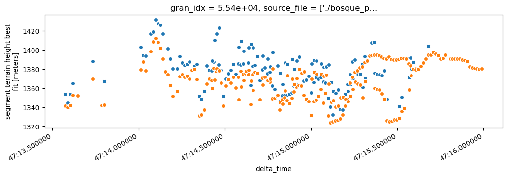

Summary

In this notebook we explored the opening and rendering ATL08 data with icepyx. We saw that icepyx will subset our downloaded data to our area of interest and also allows us to download only the variables we need. The ATL08 data has a folder-like structure with many variables to choose from. We focused on h_canopy and showed additional examples using the raw photons and h_te_best_fit for the ground height.

More information about ATL08 or icepyx can be found in: - The icepyx documentation - The Algorithm Theoretical Basis Document (ATBD) - Neuenschwander et. al. 2019, Remote Sens. Env. DOI