# Modules imported separately - not available at the time of the workshop managed environment
#!pip install --user xvec
#!pip install --user shap
#!pip install --user xgboostBIOSPACE25 Workshop:
Harnessing analysis tools for biodiversity applications using field, airborne, and orbital remote sensing data from NASA’s BioSCAPE campaign
Michele Thornton (NASA Earthdata), Rupesh Shrestha (NASA Earthdata), Erin Hestir-PI (UC Merced), Adam Wilson-PI (University at Buffalo), Jasper Slingsby-PI (University of Cape Town), Anabelle Cardoso-PM (University of Cape Town, University at Buffalo)
Date: February 12, 2025, Frascati (Rome), Italy

Tutorial: Mapping Invasive Species Using Supervised Machine Learning and AVIRIS-NG
Overview
In this notebook, we will use existing data of verified land cover and alien species locations to extract spectra from AVIRIS NG surface reflectance data.
This Notebook borrows heavily from an earlier BioSCape Workshop Notebook, but with updates to reading and analysis of AVIRIS-NG netCDF file formats.
Learning Objectives
- Understand how to inspect and prepare data for machine learning models
- Train and interpret a machine learning model
- Apply a trained model to AVIRIS imagery to create alien species maps
Load Python Modules
from os import path
import geopandas as gpd
import s3fs
import pandas as pd
import xarray as xr
from shapely.geometry import box, mapping
import rioxarray as riox
import numpy as np
import netCDF4 as nc
import hvplot.xarray
import holoviews as hv
import xvec
import shap
import xgboost
import matplotlib.pyplot as plt
from dask.diagnostics import ProgressBar
import warnings
#our functions
from utils import get_first_xr
warnings.filterwarnings('ignore')
hvplot.extension('bokeh')Explore Sample Land Type Plot-Level Data
For plot-level training data, we will use a small dataset over the Cape Town Peninsula of South Africa of manually collected invasive plant and land cover label - ct_invasive.gpkg
# let's first create a DataFrame and assign labels to each class
label_df = pd.DataFrame({'LandType': ['Bare ground/Rock','Mature Fynbos',
'Recently Burnt Fynbos', 'Wetland',
'Forest', 'Pine', 'Eucalyptus' , 'Wattle', 'Water'],
'class': ['0','1','2','3','4','5','6','7','8']})
label_df| LandType | class | |
|---|---|---|
| 0 | Bare ground/Rock | 0 |
| 1 | Mature Fynbos | 1 |
| 2 | Recently Burnt Fynbos | 2 |
| 3 | Wetland | 3 |
| 4 | Forest | 4 |
| 5 | Pine | 5 |
| 6 | Eucalyptus | 6 |
| 7 | Wattle | 7 |
| 8 | Water | 8 |
# Now let's open the dataset, project to the South African UTM projection also used by the AVIRIS-NG airborne data, and merge it with the label data frame created above.
class_data = gpd.read_file('data/ct_invasive.gpkg')
# class_data.crs
class_data_utm = (class_data
.to_crs("EPSG:32734")
.merge(label_df, on='class', how='left')
)
class_data_utm| class | group | geometry | LandType | |
|---|---|---|---|---|
| 0 | 0 | 2 | POINT (264211.767 6198008.161) | Bare ground/Rock |
| 1 | 0 | 1 | POINT (257698.443 6240453.544) | Bare ground/Rock |
| 2 | 0 | 1 | POINT (260264.755 6239108.581) | Bare ground/Rock |
| 3 | 0 | 1 | POINT (258793.622 6239111.697) | Bare ground/Rock |
| 4 | 0 | 1 | POINT (261938.819 6238865.583) | Bare ground/Rock |
| ... | ... | ... | ... | ... |
| 314 | 7 | 2 | POINT (262122.203 6228661.57) | Wattle |
| 315 | 3 | 1 | POINT (262105.078 6228827.113) | Wetland |
| 316 | 3 | 1 | POINT (262316.257 6228870.308) | Wetland |
| 317 | 7 | 1 | POINT (262822.284 6241735.006) | Wattle |
| 318 | 7 | 1 | POINT (262935.024 6241659.615) | Wattle |
319 rows × 4 columns
Summarize and Visualize the Land Types
# examine the number of plots of each land type
class_data_utm.groupby(['LandType']).size()LandType
Bare ground/Rock 32
Eucalyptus 30
Forest 34
Mature Fynbos 44
Pine 36
Recently Burnt Fynbos 32
Water 32
Wattle 24
Wetland 55
dtype: int64# The group class will be used to determine training and test data
class_data_utm.groupby(['group']).size()group
1 254
2 65
dtype: int64# Let's visualize the plot data in an interactive map, with color by class, using a Google satellite basemap
map = class_data_utm[['LandType', 'geometry']].explore('LandType', tiles='https://mt1.google.com/vt/lyrs=s&x={x}&y={y}&z={z}', attr='Google')
mapMake this Notebook Trusted to load map: File -> Trust Notebook
AVIRIS-NG Data over Cape Town Peninsula
There is a coverage file that has the bounding box of each AVIRIS-NG flight scene made available by the BioSCape Science Team. - ANG_Coverage.geojson
Scenes are provided as smaller sections within each flight line. The data for each scene within a flight line is seamless to adjacent scenes.
# read and plot the AVNG coverage file
AVNG_Coverage = gpd.read_file('data/ANGv2_Coverage.geojson', driver='GeoJSON')
AVNG_Coverage.keys()Index(['fid', 'RFL s3', 'end_time', 'geometry'], dtype='object')- note, for this workshop, that the ‘RFL s3’ field was pre-populated in the geojson file and points to S3 buckets within a BioSCape SMCE. Once BioSCape AVIRIS-NG data are published, this should be updated to point to NASA Earthdata S3 buckets.
- we’ll use the s3 file list in an upcoming code block
AVNG_Coverage.crs<Geographic 2D CRS: EPSG:4326>
Name: WGS 84
Axis Info [ellipsoidal]:
- Lat[north]: Geodetic latitude (degree)
- Lon[east]: Geodetic longitude (degree)
Area of Use:
- name: World.
- bounds: (-180.0, -90.0, 180.0, 90.0)
Datum: World Geodetic System 1984 ensemble
- Ellipsoid: WGS 84
- Prime Meridian: GreenwichAVNG_Coverage| fid | RFL s3 | end_time | geometry | |
|---|---|---|---|---|
| 0 | ang20231022t092801 | s3://bioscape-data/AVNG_V2/ang20231022t092801/... | 2023-10-22 09:28:14+00:00 | POLYGON ((18.81744 -33.05358, 18.8201 -32.9455... |
| 1 | ang20231022t092801 | s3://bioscape-data/AVNG_V2/ang20231022t092801/... | 2023-10-22 09:29:18+00:00 | POLYGON ((18.83463 -33.15597, 18.83717 -33.052... |
| 2 | ang20231022t092801 | s3://bioscape-data/AVNG_V2/ang20231022t092801/... | 2023-10-22 09:30:22+00:00 | POLYGON ((18.84821 -33.25522, 18.85068 -33.154... |
| 3 | ang20231022t092801 | s3://bioscape-data/AVNG_V2/ang20231022t092801/... | 2023-10-22 09:31:26+00:00 | POLYGON ((18.86382 -33.35258, 18.86625 -33.253... |
| 4 | ang20231022t092801 | s3://bioscape-data/AVNG_V2/ang20231022t092801/... | 2023-10-22 09:32:30+00:00 | POLYGON ((18.88141 -33.45065, 18.88384 -33.350... |
| ... | ... | ... | ... | ... |
| 3622 | ang20231126t114819 | s3://bioscape-data/AVNG_V2/ang20231126t114819/... | 2023-11-26 11:49:07+00:00 | POLYGON ((18.86453 -34.26282, 18.86562 -34.219... |
| 3623 | ang20231126t114819 | s3://bioscape-data/AVNG_V2/ang20231126t114819/... | 2023-11-26 11:49:39+00:00 | POLYGON ((18.90851 -34.29142, 18.90953 -34.250... |
| 3624 | ang20231126t114819 | s3://bioscape-data/AVNG_V2/ang20231126t114819/... | 2023-11-26 11:50:11+00:00 | POLYGON ((18.95306 -34.32059, 18.95406 -34.279... |
| 3625 | ang20231126t114819 | s3://bioscape-data/AVNG_V2/ang20231126t114819/... | 2023-11-26 11:50:43+00:00 | POLYGON ((18.99838 -34.35129, 18.99937 -34.309... |
| 3626 | ang20231126t114819 | s3://bioscape-data/AVNG_V2/ang20231126t114819/... | 2023-11-26 11:51:15+00:00 | POLYGON ((19.07408 -34.401, 19.07551 -34.33891... |
3627 rows × 4 columns
# Let's visualize the plot data in an interactive map, with color by class, using a Google satellite basemap
map = AVNG_Coverage[['fid', 'geometry']].explore(tiles='https://mt1.google.com/vt/lyrs=s&x={x}&y={y}&z={z}', attr='Google')
#map = AVNG_Coverage[['fid', 'geometry']].explore('fid')
mapMake this Notebook Trusted to load map: File -> Trust Notebook
AVIRIS-NG Principle Investigator Researchers are finalizing formats and standards of AVIRIS-NG airborne radiance and reflectance files. When finalized, the data will be published to into NASA Earthdata.
For now, JPL provides preliminatry AVIRIS-NG data here. Once finalized, AVIRIS-NG data from the BioSCape Campaign will be available from NASA Earthdata Cloud Storage.
Select the AVIRIS-NG Flight Line data to selected parameters and create lists to use later
For our analysis demonstration in this Notebook, we’ll narrow the flight lines to the area of the Cape Penisula and for flights that took place on 2023-11-09. - the Python GeoDataFrame.to_crs method Transform geometries to a new coordinate reference system.
# temporal filter: filter dates to between midnight on 2023-11-09 and 23:59:59 on 2023-11-09
AVNG_CP = AVNG_Coverage[(AVNG_Coverage['end_time'] >= '2023-11-09 00:00:00') & (AVNG_Coverage['end_time'] <= '2023-11-09 23:59:59')]
AVNG_CP = AVNG_CP.to_crs("EPSG:32734")
#keep only AVNG_CP that spatially intersects with class_data
AVNG_CP = AVNG_CP[AVNG_CP.intersects(class_data_utm.unary_union)]
#AVNG_CP
# write the AVBG_CP fields 'RFL s3' and 'geometry' to lists
files_s3 = AVNG_CP['RFL s3'].tolist()
files_AVNG_geo = AVNG_CP['geometry'].tolist()
files_AVNG_geo
#Visualize the selected flight lines
#m = AVNG_CP[['fid','geometry']].explore('fid')
m = AVNG_CP[['fid', 'geometry']].explore('fid', tiles='https://mt1.google.com/vt/lyrs=s&x={x}&y={y}&z={z}', attr='Google')
#explore('LandType', tiles='https://mt1.google.com/vt/lyrs=s&x={x}&y={y}&z={z}', attr='Google')
mMake this Notebook Trusted to load map: File -> Trust Notebook
AVNG_CP.to_file('AVNG_CP.geojson', driver='GeoJSON')AVNG_CP.crs<Projected CRS: EPSG:32734>
Name: WGS 84 / UTM zone 34S
Axis Info [cartesian]:
- E[east]: Easting (metre)
- N[north]: Northing (metre)
Area of Use:
- name: Between 18°E and 24°E, southern hemisphere between 80°S and equator, onshore and offshore. Angola. Botswana. Democratic Republic of the Congo (Zaire). Namibia. South Africa. Zambia.
- bounds: (18.0, -80.0, 24.0, 0.0)
Coordinate Operation:
- name: UTM zone 34S
- method: Transverse Mercator
Datum: World Geodetic System 1984 ensemble
- Ellipsoid: WGS 84
- Prime Meridian: Greenwichprint(AVNG_CP['fid'])1561 ang20231109t125547
1563 ang20231109t125547
1564 ang20231109t130728
1565 ang20231109t130728
1566 ang20231109t130728
1567 ang20231109t130728
1568 ang20231109t130728
1569 ang20231109t130728
1574 ang20231109t131923
1575 ang20231109t131923
1576 ang20231109t131923
1577 ang20231109t131923
1578 ang20231109t131923
1579 ang20231109t131923
1580 ang20231109t131923
1581 ang20231109t133124
1582 ang20231109t133124
1583 ang20231109t133124
1584 ang20231109t133124
1585 ang20231109t133124
1586 ang20231109t133124
1587 ang20231109t133124
1591 ang20231109t134249
1592 ang20231109t134249
1593 ang20231109t134249
1594 ang20231109t134249
1595 ang20231109t134249
1596 ang20231109t134249
1598 ang20231109t135449
1599 ang20231109t135449
1600 ang20231109t135449
1601 ang20231109t135449
1602 ang20231109t135449
1608 ang20231109t140547
1609 ang20231109t140547
1610 ang20231109t140547
1617 ang20231109t141759
Name: fid, dtype: object# Let's print a full file path for a Reflectance file in netCDF format. Recall that this S3 path in within the BioSCape SMCE.
files_s3[26]'s3://bioscape-data/AVNG_V2/ang20231109t134249/ang20231109t134249_006/ang20231109t134249_006_L2A_OE_0b4f48b4_RFL_ORT.nc'The AVIRIS-NG files are also in S3 buckets in a BioSCape Science Managed Cloud Environment (SMCE).
- SMCE’s support NASA Funded researchers by providing a secure hub to store and analyze data. These SMCE’s are in AWS US-West. For demonstrative puposes, Workshop instructors (but not participants) are able to access these files. Once BioSCape AVIRIS-NG are published, this can be adapated to Earthdata S3 links.
- The AVIRIS-NG data are accessed through the BioSCape SMCE in the following block. Once BioSCape AVIRIS-NG data are published into NASA Earthdata Cloud, this Notebook should be updated to demonstrate
# Using BioSCape AWS Credentials to acces BioSCape SMCE. keys and token are removed for notebook publication
import s3fs
secret_key=''
access_key=''
token =''
fs = s3fs.S3FileSystem(anon=False,
secret=secret_key,
key=access_key,
token=token)Explore the BioSCape S3 Data Holdings
We’ll demonstrate here how to explore a file-like system on an S3 Bucket using the BioSCape SMCE arrangement. - S3 = Amazon Simple Storage Service (S3) is a cloud storage service that allows users to store and retrieve data - S3 Bucket = Buckets are the basic containers that hold data. Buckets can be likened to file folders and object storage - S3Fs is a Pythonic open source tool that mounts S3 object storage locally. S3Fs provides a filesystem-like interface for accessing objects on S3. >import s3fs > >fs = s3fs.S3FileSystem(anon=False)
- The top-level class
S3FileSystemholds connection information and allows typical file-system style operations likels,cp,mvlsis a UNIX command to list computer files and directories
fs.ls('bioscape-data/')['bioscape-data/AVNG_V2',
'bioscape-data/BioSCapeVegPolys2023_10_18.geoparquet',
'bioscape-data/LVIS',
'bioscape-data/PRISM',
'bioscape-data/bioscape_avng_v2.yaml']#fs.ls('bioscape-data/AVNG_V2/')fs.ls('bioscape-data/AVNG_V2/ang20231109t133124/ang20231109t133124_005')['bioscape-data/AVNG_V2/ang20231109t133124/ang20231109t133124_005/ang20231109t133124_005_L1B_ORT_fb78102f_OBS.json',
'bioscape-data/AVNG_V2/ang20231109t133124/ang20231109t133124_005/ang20231109t133124_005_L1B_ORT_fb78102f_OBS.nc',
'bioscape-data/AVNG_V2/ang20231109t133124/ang20231109t133124_005/ang20231109t133124_005_L1B_RDN_4a3c998e_RDN.json',
'bioscape-data/AVNG_V2/ang20231109t133124/ang20231109t133124_005/ang20231109t133124_005_L1B_RDN_4a3c998e_RDN.nc',
'bioscape-data/AVNG_V2/ang20231109t133124/ang20231109t133124_005/ang20231109t133124_005_L2A_OE_0b4f48b4_RFL_ORT.json',
'bioscape-data/AVNG_V2/ang20231109t133124/ang20231109t133124_005/ang20231109t133124_005_L2A_OE_0b4f48b4_RFL_ORT.nc']File Naming Conventions provide information about each flight line, scene, and data type.
L1Bare AVIRIS-NG Surface RadianceL2Aare AVIRIS-NG Surface Reflectance
| Dataset | Description |
|---|---|
| *_OBS.nc | Orthocorrected observational parameters |
| *_RDN.nc | Calibrated Radiance netCDF file (3 band) |
| *_RFL_ORT.nc | Reflectance netCDF file (425 band) |
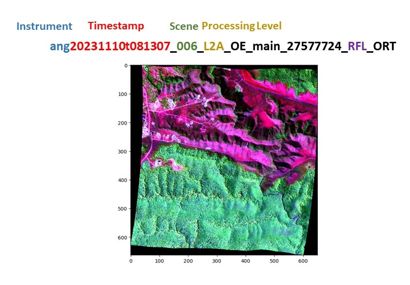
Single AVIRIS-NG flight scene Reflectance file ang20231109t133124_005_L2A_OE_0b4f48b4_RFL_ORT.nc
- For the workshop, we will ask participants to download one scence from JPL into the 2i2c Hub environment provided for workshop participants
- One file can quickly be downloaded to the participants unique environment using this wget command line
wget https://popo.jpl.nasa.gov/pub/bioscape_netCDF/rfl/ang20231109t133124_005_L2A_OE_0b4f48b4_RFL_ORT.nc -P /home/jovyan/2025-biospace/tutorial/avirisng/data/ang
Open a single AVIRIS-NG Reflectance file to inspect the data
xarrayis an open source project and Python package that introduces labels in the form of dimensions, coordinates, and attributes on top of raw NumPy-like arrays
# - we're using **`S3Fs`** to mount S3 object storage locally
## Sample code to open a file from an S3 bucket using S3Fs
#rfl_netcdf = xr.open_datatree(fs.open(files_s3[26], 'rb'),
# engine='h5netcdf', chunks={})
# For this workshop, we're using a local AVIRIS-NG scence
rfl_netcdf_2i2c = 'data/ang/ang20231109t134249_006_L2A_OE_0b4f48b4_RFL_ORT.nc'
rfl_netcdf_2i2c'data/ang/ang20231109t134249_006_L2A_OE_0b4f48b4_RFL_ORT.nc'#rfl_netcdf = xr.open_datatree(fs.open(files_s3[26], 'rb'),
# engine='h5netcdf', chunks={})
rfl_netcdf = xr.open_datatree(rfl_netcdf_2i2c,
engine='h5netcdf', chunks={})
rfl_netcdf = rfl_netcdf.reflectance.to_dataset()
rfl_netcdf = rfl_netcdf.reflectance.where(rfl_netcdf.reflectance>0)
rfl_netcdf<xarray.DataArray 'reflectance' (wavelength: 425, northing: 1744, easting: 636)> Size: 2GB
dask.array<where, shape=(425, 1744, 636), dtype=float32, chunksize=(10, 256, 256), chunktype=numpy.ndarray>
Coordinates:
* easting (easting) float64 5kB 8.109e+05 8.109e+05 ... 8.141e+05
* northing (northing) float64 14kB 6.216e+06 6.216e+06 ... 6.207e+06
* wavelength (wavelength) float32 2kB 377.2 382.2 ... 2.496e+03 2.501e+03
Attributes:
_QuantizeBitGroomNumberOfSignificantDigits: 5
long_name: Surface hemispherical direct...
grid_mapping: transverse_mercator
orthorectified: TruePlot a true color image
h = rfl_netcdf.sel(wavelength=[660, 570, 480], method="nearest").hvplot.rgb('easting', 'northing',
rasterize=True, data_aspect=1,
bands='wavelength', frame_width=400)
hPlot just a red reflectance
h = rfl_netcdf.sel({'wavelength': 660},method='nearest').hvplot('easting', 'northing',
rasterize=True, data_aspect=1,
cmap='magma',frame_width=400,clim=(0,0.3))
hExtract Spectra for each Land Plot
Now that we are familiar with the data, we want to get the AVIRIS spectra at each label location. Below is a function that does this and returns the result as a xarray
Recall some files we created earlier: - files_s3 = list; S3 netCDF files directories from the Cape Penisula subset area - files_AVNG_geo = list; coordinates of bounding boxes of the flight line scenes from the Cape Penisula area - class_data_utm = gpd; Cape Penisula Land Types with UTM geography
#the function takes a filepath to a file on s3, and the point locations for extraction
#this function requires hitting files on the BioSCape SMCE
def extract_points(s3uri, geof, points):
ds = xr.open_datatree(fs.open(s3uri, 'rb'), decode_coords='all',
engine='h5netcdf', chunks='auto')
# Clip the raw data to the bounding box
points = points.clip(geof)
print(f'got {points.shape[0]} point from {s3uri}')
points = points.to_crs(ds.transverse_mercator.crs_wkt)
# Extract points
#extracted = ds.to_dataset().xvec.extract_points(points['geometry'], x_coords="easting", y_coords="northing",index=True)
extracted = ds.reflectance.to_dataset().xvec.extract_points(points['geometry'],
x_coords="easting",
y_coords="northing",
index=True)
return extractedWhen we call the function, we’ll iterate through the list of files (files_s3). Each file will overlap with several land class points.
ds_all = [extract_points(file, geo, class_data_utm) for file, geo in zip(files_s3, files_AVNG_geo)]
ds_all = xr.concat(ds_all, dim='file')got 2 point from s3://bioscape-data/AVNG_V2/ang20231109t125547/ang20231109t125547_005/ang20231109t125547_005_L2A_OE_0b4f48b4_RFL_ORT.nc
got 7 point from s3://bioscape-data/AVNG_V2/ang20231109t125547/ang20231109t125547_007/ang20231109t125547_007_L2A_OE_0b4f48b4_RFL_ORT.nc
got 11 point from s3://bioscape-data/AVNG_V2/ang20231109t130728/ang20231109t130728_000/ang20231109t130728_000_L2A_OE_0b4f48b4_RFL_ORT.nc
got 12 point from s3://bioscape-data/AVNG_V2/ang20231109t130728/ang20231109t130728_001/ang20231109t130728_001_L2A_OE_0b4f48b4_RFL_ORT.nc
got 4 point from s3://bioscape-data/AVNG_V2/ang20231109t130728/ang20231109t130728_002/ang20231109t130728_002_L2A_OE_0b4f48b4_RFL_ORT.nc
got 20 point from s3://bioscape-data/AVNG_V2/ang20231109t130728/ang20231109t130728_003/ang20231109t130728_003_L2A_OE_0b4f48b4_RFL_ORT.nc
got 1 point from s3://bioscape-data/AVNG_V2/ang20231109t130728/ang20231109t130728_004/ang20231109t130728_004_L2A_OE_0b4f48b4_RFL_ORT.nc
got 19 point from s3://bioscape-data/AVNG_V2/ang20231109t130728/ang20231109t130728_005/ang20231109t130728_005_L2A_OE_0b4f48b4_RFL_ORT.nc
got 2 point from s3://bioscape-data/AVNG_V2/ang20231109t131923/ang20231109t131923_002/ang20231109t131923_002_L2A_OE_0b4f48b4_RFL_ORT.nc
got 45 point from s3://bioscape-data/AVNG_V2/ang20231109t131923/ang20231109t131923_003/ang20231109t131923_003_L2A_OE_0b4f48b4_RFL_ORT.nc
got 9 point from s3://bioscape-data/AVNG_V2/ang20231109t131923/ang20231109t131923_004/ang20231109t131923_004_L2A_OE_0b4f48b4_RFL_ORT.nc
got 29 point from s3://bioscape-data/AVNG_V2/ang20231109t131923/ang20231109t131923_005/ang20231109t131923_005_L2A_OE_0b4f48b4_RFL_ORT.nc
got 9 point from s3://bioscape-data/AVNG_V2/ang20231109t131923/ang20231109t131923_006/ang20231109t131923_006_L2A_OE_0b4f48b4_RFL_ORT.nc
got 21 point from s3://bioscape-data/AVNG_V2/ang20231109t131923/ang20231109t131923_007/ang20231109t131923_007_L2A_OE_0b4f48b4_RFL_ORT.nc
got 5 point from s3://bioscape-data/AVNG_V2/ang20231109t131923/ang20231109t131923_008/ang20231109t131923_008_L2A_OE_0b4f48b4_RFL_ORT.nc
got 5 point from s3://bioscape-data/AVNG_V2/ang20231109t133124/ang20231109t133124_000/ang20231109t133124_000_L2A_OE_0b4f48b4_RFL_ORT.nc
got 14 point from s3://bioscape-data/AVNG_V2/ang20231109t133124/ang20231109t133124_001/ang20231109t133124_001_L2A_OE_0b4f48b4_RFL_ORT.nc
got 9 point from s3://bioscape-data/AVNG_V2/ang20231109t133124/ang20231109t133124_002/ang20231109t133124_002_L2A_OE_0b4f48b4_RFL_ORT.nc
got 26 point from s3://bioscape-data/AVNG_V2/ang20231109t133124/ang20231109t133124_003/ang20231109t133124_003_L2A_OE_0b4f48b4_RFL_ORT.nc
got 42 point from s3://bioscape-data/AVNG_V2/ang20231109t133124/ang20231109t133124_004/ang20231109t133124_004_L2A_OE_0b4f48b4_RFL_ORT.nc
got 34 point from s3://bioscape-data/AVNG_V2/ang20231109t133124/ang20231109t133124_005/ang20231109t133124_005_L2A_OE_0b4f48b4_RFL_ORT.nc
got 3 point from s3://bioscape-data/AVNG_V2/ang20231109t133124/ang20231109t133124_006/ang20231109t133124_006_L2A_OE_0b4f48b4_RFL_ORT.nc
got 3 point from s3://bioscape-data/AVNG_V2/ang20231109t134249/ang20231109t134249_002/ang20231109t134249_002_L2A_OE_0b4f48b4_RFL_ORT.nc
got 40 point from s3://bioscape-data/AVNG_V2/ang20231109t134249/ang20231109t134249_003/ang20231109t134249_003_L2A_OE_0b4f48b4_RFL_ORT.nc
got 34 point from s3://bioscape-data/AVNG_V2/ang20231109t134249/ang20231109t134249_004/ang20231109t134249_004_L2A_OE_0b4f48b4_RFL_ORT.nc
got 13 point from s3://bioscape-data/AVNG_V2/ang20231109t134249/ang20231109t134249_005/ang20231109t134249_005_L2A_OE_0b4f48b4_RFL_ORT.nc
got 21 point from s3://bioscape-data/AVNG_V2/ang20231109t134249/ang20231109t134249_006/ang20231109t134249_006_L2A_OE_0b4f48b4_RFL_ORT.nc
got 12 point from s3://bioscape-data/AVNG_V2/ang20231109t134249/ang20231109t134249_007/ang20231109t134249_007_L2A_OE_0b4f48b4_RFL_ORT.nc
got 10 point from s3://bioscape-data/AVNG_V2/ang20231109t135449/ang20231109t135449_001/ang20231109t135449_001_L2A_OE_0b4f48b4_RFL_ORT.nc
got 18 point from s3://bioscape-data/AVNG_V2/ang20231109t135449/ang20231109t135449_002/ang20231109t135449_002_L2A_OE_0b4f48b4_RFL_ORT.nc
got 12 point from s3://bioscape-data/AVNG_V2/ang20231109t135449/ang20231109t135449_003/ang20231109t135449_003_L2A_OE_0b4f48b4_RFL_ORT.nc
got 12 point from s3://bioscape-data/AVNG_V2/ang20231109t135449/ang20231109t135449_004/ang20231109t135449_004_L2A_OE_0b4f48b4_RFL_ORT.nc
got 12 point from s3://bioscape-data/AVNG_V2/ang20231109t135449/ang20231109t135449_005/ang20231109t135449_005_L2A_OE_0b4f48b4_RFL_ORT.nc
got 7 point from s3://bioscape-data/AVNG_V2/ang20231109t140547/ang20231109t140547_004/ang20231109t140547_004_L2A_OE_0b4f48b4_RFL_ORT.nc
got 5 point from s3://bioscape-data/AVNG_V2/ang20231109t140547/ang20231109t140547_005/ang20231109t140547_005_L2A_OE_0b4f48b4_RFL_ORT.nc
got 10 point from s3://bioscape-data/AVNG_V2/ang20231109t140547/ang20231109t140547_006/ang20231109t140547_006_L2A_OE_0b4f48b4_RFL_ORT.nc
got 2 point from s3://bioscape-data/AVNG_V2/ang20231109t141759/ang20231109t141759_004/ang20231109t141759_004_L2A_OE_0b4f48b4_RFL_ORT.ncds_all<xarray.Dataset> Size: 20MB
Dimensions: (file: 37, wavelength: 425, geometry: 319)
Coordinates:
* wavelength (wavelength) float32 2kB 377.2 382.2 ... 2.496e+03 2.501e+03
* geometry (geometry) object 3kB POINT (820376.8345556275 6221215.53145...
index (file, geometry) float64 94kB 241.0 240.0 nan ... nan nan nan
Dimensions without coordinates: file
Data variables:
fwhm (file, wavelength) float32 63kB dask.array<chunksize=(1, 425), meta=np.ndarray>
reflectance (file, wavelength, geometry) float32 20MB dask.array<chunksize=(1, 30, 1), meta=np.ndarray>
Indexes:
geometry GeometryIndex (crs=EPSG:32733)Because some points are covered by multiple AVIRIS scenes, some points have multiple spectra for each location, and thus we have an extra dim in this. We will simply extract the first valid reflectance measurement for each geometry. We have a custom function to do this get_first_xr()
ds = get_first_xr(ds_all)
ds<xarray.Dataset> Size: 549kB
Dimensions: (wavelength: 425, index: 319)
Coordinates:
* wavelength (wavelength) float32 2kB 377.2 382.2 ... 2.496e+03 2.501e+03
geometry (index) object 3kB POINT (820376.8345556275 6221215.53145171...
* index (index) int64 3kB 241 240 18 17 19 20 ... 82 289 246 52 51 137
Data variables:
reflectance (index, wavelength) float32 542kB dask.array<chunksize=(1, 30), meta=np.ndarray>This data set just has the spectra. We need to merge with point data to add labels
class_xr =class_data_utm[['class','group']].to_xarray()
ds = ds.merge(class_xr.astype(int),join='left')
ds<xarray.Dataset> Size: 554kB
Dimensions: (wavelength: 425, index: 319)
Coordinates:
* wavelength (wavelength) float32 2kB 377.2 382.2 ... 2.496e+03 2.501e+03
* index (index) int64 3kB 241 240 18 17 19 20 ... 82 289 246 52 51 137
geometry (index) object 3kB POINT (820376.8345556275 6221215.53145171...
Data variables:
reflectance (index, wavelength) float32 542kB dask.array<chunksize=(1, 30), meta=np.ndarray>
class (index) int64 3kB 8 8 0 0 1 1 8 3 8 1 4 ... 6 1 1 1 3 8 8 2 2 5
group (index) int64 3kB 1 1 1 1 1 1 1 1 1 1 1 ... 1 1 1 2 2 2 1 1 1 1We have defined all the operations we want, but becasue of xarrays lazy compution, the calculations have not yet been done. We will now force it to perform this calculations. We want to keep the result in chunks, so we use .persist() and not .compute(). This should take approx 2 - 3 mins
## DUE TO RUN TIME LENGTH, WE WILL NOT RUN THIS IN THE WORKSHOP - For this workshop, we HAVE SAVED THIS OUTPUT (dsp.nc) and it is available FOR NEXT STEP
# with ProgressBar():
# dsp = ds.persist()dsp = xr.open_dataset('dsp.nc')
dsp<xarray.Dataset> Size: 552kB
Dimensions: (wavelength: 425, index: 319)
Coordinates:
* wavelength (wavelength) float32 2kB 377.2 382.2 ... 2.496e+03 2.501e+03
* index (index) int64 3kB 241 240 18 17 19 20 ... 82 289 246 52 51 137
Data variables:
reflectance (index, wavelength) float32 542kB ...
class (index) int64 3kB ...
group (index) int64 3kB ...Inspect AVIRIS spectra
# recall the class types
label_df| LandType | class | |
|---|---|---|
| 0 | Bare ground/Rock | 0 |
| 1 | Mature Fynbos | 1 |
| 2 | Recently Burnt Fynbos | 2 |
| 3 | Wetland | 3 |
| 4 | Forest | 4 |
| 5 | Pine | 5 |
| 6 | Eucalyptus | 6 |
| 7 | Wattle | 7 |
| 8 | Water | 8 |
dsp_plot = dsp.where(dsp['class']==5, drop=True)
h = dsp_plot['reflectance'].hvplot.line(x='wavelength',by='index',
color='green', alpha=0.5,legend=False)
hAt this point in a real machine learning workflow, you should closely inspect the spectra you have for each class. Do they make sense? Are there some spectra that look weird? You should re-evaluate your data to make sure that the assigned labels are true. This is a very important step
Prep data for ML model
As you will know, not all of the wavelengths in the data are of equal quality, some will be degraded by atmospheric water absorption features or other factors. We should remove the bands from the analysis that we are not confident of. Probably the best way to do this is to use the uncertainties provided along with the reflectance files. We will simply use some prior knowledge to screen out the worst bands.
wavelengths_to_drop = dsp.wavelength.where(
(dsp.wavelength < 450) |
(dsp.wavelength >= 1340) & (dsp.wavelength <= 1480) |
(dsp.wavelength >= 1800) & (dsp.wavelength <= 1980) |
(dsp.wavelength > 2400), drop=True
)
# Use drop_sel() to remove those specific wavelength ranges
dsp = dsp.drop_sel(wavelength=wavelengths_to_drop)
mask = (dsp['reflectance'] > -1).all(dim='wavelength') # Create a mask where all values along 'z' are non-negative
dsp = dsp.sel(index=mask)
dsp<xarray.Dataset> Size: 377kB
Dimensions: (wavelength: 325, index: 284)
Coordinates:
* wavelength (wavelength) float32 1kB 452.3 457.3 ... 2.391e+03 2.396e+03
* index (index) int64 2kB 241 240 18 17 19 20 ... 40 289 246 52 51 137
Data variables:
reflectance (index, wavelength) float32 369kB 0.02946 0.02944 ... 0.01413
class (index) int64 2kB 8 8 0 0 1 1 3 8 1 4 3 ... 6 6 1 1 1 8 8 2 2 5
group (index) int64 2kB ...Next we will normalize the data, there are a number of difference normalizations to try. In a ML workflow you should try a few and see which work best. We will only use a Brightness Normalization. In essence, we scale the reflectance of each wavelength by the total brightness of the spectra. This retains info on important shape features and relative reflectance, and removes info on absolute reflectance.
# Calculate the L2 norm along the 'wavelength' dimension
l2_norm = np.sqrt((dsp['reflectance'] ** 2).sum(dim='wavelength'))
# Normalize the reflectance by dividing by the L2 norm
dsp['reflectance'] = dsp['reflectance'] / l2_normPlot the new, clean spectra
dsp_norm_plot = dsp.where(dsp['class']==5, drop=True)
h = dsp_norm_plot['reflectance'].hvplot.line(x='wavelength',by='index',
color='green',ylim=(-0.01,0.2),alpha=0.5,legend=False)
hTrain and evaluate the ML model
We will be using a model called xgboost. There are many, many different kinds of ML models. xgboost is a class of models called gradient boosted trees, related to random forests. When used for classification, random forests work by creating multiple decision trees, each trained on a random subset of the data and features, and then averaging their predictions to improve accuracy and reduce overfitting. Gradient boosted trees differ in that they build trees sequentially, with each new tree focusing on correcting the errors of the previous ones. This sequential approach allows xgboost to create highly accurate models by iteratively refining predictions and addressing the weaknesses of earlier trees.
Import the Machine Learning libraries we will use.
import xgboost as xgb
from sklearn.model_selection import GridSearchCV
from sklearn.metrics import accuracy_score, f1_score, precision_score, recall_score, confusion_matrix, ConfusionMatrixDisplayOur dataset has a label indicating which set (training or test), our data belong to. We wil use this to split it
# recall groups
class_data_utm.groupby(['group']).size()group
1 254
2 65
dtype: int64class_data_utm.crs<Projected CRS: EPSG:32734>
Name: WGS 84 / UTM zone 34S
Axis Info [cartesian]:
- E[east]: Easting (metre)
- N[north]: Northing (metre)
Area of Use:
- name: Between 18°E and 24°E, southern hemisphere between 80°S and equator, onshore and offshore. Angola. Botswana. Democratic Republic of the Congo (Zaire). Namibia. South Africa. Zambia.
- bounds: (18.0, -80.0, 24.0, 0.0)
Coordinate Operation:
- name: UTM zone 34S
- method: Transverse Mercator
Datum: World Geodetic System 1984 ensemble
- Ellipsoid: WGS 84
- Prime Meridian: Greenwichdtrain = dsp.where(dsp['group']==1,drop=True)
dtest = dsp.where(dsp['group']==2,drop=True)
#create separte datasets for labels and features
y_train = dtrain['class'].values.astype(int)
y_test = dtest['class'].values.astype(int)
X_train = dtrain['reflectance'].values
X_test = dtest['reflectance'].valuesTrain ML model
The steps we will go through to train the model are:
First, we define the hyperparameter grid. Initially, we set up a comprehensive grid (param_grid) with multiple values for several hyperparameters of the XGBoost model.
Next, we create an XGBoost classifier object using the XGBClassifier class from the XGBoost library.
We then set up the GridSearchCV object using our defined XGBoost model and the hyperparameter grid. GridSearchCV allows us to perform an exhaustive search over the specified hyperparameter values to find the optimal combination that results in the best model performance. We choose a 5-fold cross-validation strategy (cv=5), meaning we split our training data into five subsets to validate the model’s performance across different data splits. We use accuracy as our scoring metric to evaluate the models.
After setting up the grid search, we fit the GridSearchCV object to our training data (X_train and y_train). This process involves training multiple models with different hyperparameter combinations and evaluating their performance using cross-validation. Our goal is to identify the set of hyperparameters that yields the highest accuracy.
Once the grid search completes, we print out the best set of hyperparameters and the corresponding best score. The grid_search.best_params_ attribute provides the combination of hyperparameters that achieved the highest cross-validation accuracy, while the grid_search.best_score_ attribute shows the corresponding accuracy score. Finally, we extract the best model (best_model) from the grid search results. This model is trained with the optimal hyperparameters and is ready for making predictions or further analysis in our classification task.
This will take approx 30 seconds
# Define the hyperparameter grid
param_grid = {
'max_depth': [5],
'learning_rate': [0.1],
'subsample': [0.75],
'n_estimators' : [50,100]
}
# Create the XGBoost model object
xgb_model = xgb.XGBClassifier(tree_method='hist')
# Create the GridSearchCV object
grid_search = GridSearchCV(xgb_model, param_grid, cv=5, scoring='accuracy')
# Fit the GridSearchCV object to the training data
grid_search.fit(X_train, y_train)
# Print the best set of hyperparameters and the corresponding score
print("Best set of hyperparameters: ", grid_search.best_params_)
print("Best score: ", grid_search.best_score_)
best_model = grid_search.best_estimator_Best set of hyperparameters: {'learning_rate': 0.1, 'max_depth': 5, 'n_estimators': 100, 'subsample': 0.75}
Best score: 0.6711111111111111Evaluate model performance
We will use our best model to predict the classes of the test data Then, we calculate the F1 score using f1_score, which balances precision and recall, and print it to evaluate overall performance.
Next, we assess how well the model performs for predicting Pine trees by calculating its precision and recall. Precision measures the accuracy of the positive predictions. It answers the question, “Of all the instances we labeled as Pines, how many were actually Pines?”. Recall measures the model’s ability to identify all actual positive instances. It answers the question, “Of all the actual Pines, how many did we correctly identify?”. You may also be familiar with the terms Users’ and Producers’ Accuracy. Precision = User’ Accuracy, and Recall = Producers’ Accuracy.
Finally, we create and display a confusion matrix to visualize the model’s prediction accuracy across all classes
y_pred = best_model.predict(X_test)
# Step 2: Calculate acc and F1 score for the entire dataset
acc = accuracy_score(y_test, y_pred)
print(f"Accuracy: {acc}")
f1 = f1_score(y_test, y_pred, average='weighted') # 'weighted' accounts for class imbalance
print(f"F1 Score (weighted): {f1}")
# Step 3: Calculate precision and recall for class 5 (Pine)
precision_class_5 = precision_score(y_test, y_pred, labels=[5], average='macro', zero_division=0)
recall_class_5 = recall_score(y_test, y_pred, labels=[5], average='macro', zero_division=0)
print(f"Precision for Class 5: {precision_class_5}")
print(f"Recall for Class 5: {recall_class_5}")
# Step 4: Plot the confusion matrix
conf_matrix = confusion_matrix(y_test, y_pred)
ConfusionMatrixDisplay(confusion_matrix=conf_matrix).plot()
plt.show()Accuracy: 0.6271186440677966
F1 Score (weighted): 0.6124797325196129
Precision for Class 5: 0.5
Recall for Class 5: 0.3333333333333333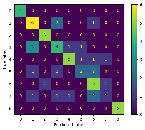
Skipping Some steps in the BioSCape Workshop Tutorial
For the length of this workshop, we cannot cover all steps that were in the BioSCape Cape Town Workshop. But links are provided here:
8.2.1.8. Interpret and understand ML model
- https://ornldaac.github.io/bioscape_workshop_sa/tutorials/Machine_Learning/Invasive_AVIRIS.html#interpret-and-understand-ml-model
Predict over an example AVIRIS scene
We now have a trained model and are ready to deploy it to generate predictions across an entire AVIRIS scene and map the distribution of invasive plants. This involves handling a large volume of data, so we need to write the code to do this intelligently. We will accomplish this by applying the .predict() method of our trained model in parallel across the chunks of the AVIRIS xarray. The model will receive one chunk at a time so that the data is not too large, but it will be able to perform this operation in parallel across multiple chunks, and therefore will not take too long.
This model was only trained on data covering natural vegetaton in the Cape Peninsula, It is important that we only predict in the areas that match our training data. We will therefore filter to scenes that cover the Cape Peninsula and mask out non-protected areas - SAPAD_2024.gpkg
#south africa protected areas
SAPAD = (gpd.read_file('data/SAPAD_2024.gpkg')
.query("SITE_TYPE!='Marine Protected Area'")
)
#SAPAD.plot()
#SAPAD.to_crs("EPSG:32734")
SAPAD.crs<Geographic 2D CRS: EPSG:4326>
Name: WGS 84
Axis Info [ellipsoidal]:
- Lat[north]: Geodetic latitude (degree)
- Lon[east]: Geodetic longitude (degree)
Area of Use:
- name: World.
- bounds: (-180.0, -90.0, 180.0, 90.0)
Datum: World Geodetic System 1984 ensemble
- Ellipsoid: WGS 84
- Prime Meridian: Greenwich# Get the bounding box of the training data
bbox = class_data_utm.total_bounds # (minx, miny, maxx, maxy)
#bbox
gdf_bbox = gpd.GeoDataFrame({'geometry': [box(*bbox)]}, crs=class_data_utm.crs) # Specify the CRS
gdf_bbox['geometry'] = gdf_bbox.buffer(500)
gdf_bbox.crs<Projected CRS: EPSG:32734>
Name: WGS 84 / UTM zone 34S
Axis Info [cartesian]:
- E[east]: Easting (metre)
- N[north]: Northing (metre)
Area of Use:
- name: Between 18°E and 24°E, southern hemisphere between 80°S and equator, onshore and offshore. Angola. Botswana. Democratic Republic of the Congo (Zaire). Namibia. South Africa. Zambia.
- bounds: (18.0, -80.0, 24.0, 0.0)
Coordinate Operation:
- name: UTM zone 34S
- method: Transverse Mercator
Datum: World Geodetic System 1984 ensemble
- Ellipsoid: WGS 84
- Prime Meridian: Greenwich#south africa protected areas
SAPAD = (gpd.read_file('data/SAPAD_2024.gpkg')
.query("SITE_TYPE!='Marine Protected Area'")
)
SAPAD = SAPAD.to_crs("EPSG:32734")
# Get the bounding box of the training data
bbox = class_data_utm.total_bounds # (minx, miny, maxx, maxy)
gdf_bbox = gpd.GeoDataFrame({'geometry': [box(*bbox)]}, crs=class_data_utm.crs) # Specify the CRS
gdf_bbox['geometry'] = gdf_bbox.buffer(500)
# protected areas that intersect with the training data
SAPAD_CT = SAPAD.overlay(gdf_bbox,how='intersection')
#keep only AVIRIS scenes that intersects with CT protected areas
AVNG_sapad = AVNG_CP[AVNG_CP.intersects(SAPAD_CT.unary_union)]
#a list of files to predict
files_sapad = AVNG_sapad['RFL s3'].tolist()
#how many files?
len(files_sapad)36m = AVNG_sapad[['fid','geometry']].explore('fid')
mMake this Notebook Trusted to load map: File -> Trust Notebook
SAPAD.keys()Index(['WDPAID', 'CUR_NME', 'WMCM_TYPE', 'MAJ_TYPE', 'SITE_TYPE', 'D_DCLAR',
'LEGAL_STAT', 'GIS_AREA', 'PROC_DOC', 'Shape_Leng', 'Shape_Area',
'geometry'],
dtype='object')#map = AVNG_Coverage[['fid', 'geometry']].explore('fid')
map = SAPAD[['SITE_TYPE', 'geometry']].explore('SITE_TYPE')
mapMake this Notebook Trusted to load map: File -> Trust Notebook
Here is the function that we will actually apply to each chunk. Simple really. The hard work is getting the data into and out of this functiON
def predict_on_chunk(chunk, model):
probabilities = model.predict_proba(chunk)
return probabilitiesNow we define the funciton that takes as input the path to the AVIRIS file and pass the data to the predict function. THhs is composed of 4 parts:
Part 1: Opens the AVIRIS data file using xarray and sets a condition to identify valid data points where reflectance values are greater than zero.
Part 2: Applies all the transformations that need to be done before the data goes to the model. It the spatial dimensions (x and y) into a single dimension, filters wavelengths, and normalizes the reflectance data.
Part 3: Applies the machine learning model to the normalized data in parallel, predicting class probabilities for each data point using xarray’s apply_ufunc method. Most of the function invloves defining what to do with the dimensions of the old dataset and the new output
Part 4: Unstacks the data to restore its original dimensions, sets spatial dimensions and coordinate reference system (CRS), clips the data, and transposes the data to match expected formats before returning the results.
def predict_xr(file,geometries):
#part 1 - opening file
#open the file
print(f'file: {file}')
ds = xr.open_datatree(rfl_netcdf_2i2c, engine='h5netcdf', decode_coords="all",
chunks='auto')
#get the geometries of the protected areas for masking
ds_crs = ds.transverse_mercator.crs_wkt
geometries = geometries.to_crs(ds_crs).geometry.apply(mapping)
#condition to use for masking no data later
condition = (ds['reflectance'] > -1).any(dim='wavelength')
#stack the data into a single dimension. This will be important for applying the model later
ds = ds.reflectance.to_dataset().stack(sample=('easting','northing'))
#part 2 - pre-processing
#remove bad wavelenghts
wavelengths_to_drop = ds.wavelength.where(
(ds.wavelength < 450) |
(ds.wavelength >= 1340) & (ds.wavelength <= 1480) |
(ds.wavelength >= 1800) & (ds.wavelength <= 1980) |
(ds.wavelength > 2400), drop=True
)
# Use drop_sel() to remove those specific wavelength ranges
ds = ds.drop_sel(wavelength=wavelengths_to_drop)
#normalise the data
l2_norm = np.sqrt((ds['reflectance'] ** 2).sum(dim='wavelength'))
ds['reflectance'] = ds['reflectance'] / l2_norm
#part 3 - apply the model over chunks
result = xr.apply_ufunc(
predict_on_chunk,
ds['reflectance'].chunk(dict(wavelength=-1)),
input_core_dims=[['wavelength']],#input dim with features
output_core_dims=[['class']], # name for the new output dim
exclude_dims=set(('wavelength',)), #dims to drop in result
output_sizes={'class': 9}, #length of the new dimension
output_dtypes=[np.float32],
dask="parallelized",
kwargs={'model': best_model}
)
#part 4 - post-processing
result = result.where((result >= 0) & (result <= 1), np.nan) #valid values
result = result.unstack('sample') #remove the stack
result = result.rio.set_spatial_dims(x_dim='easting',y_dim='northing') #set the spatial dims
result = result.rio.write_crs(ds_crs) #set the CRS
result = result.rio.clip(geometries) #clip to the protected areas and no data
result = result.transpose('class', 'northing', 'easting') #transpose the data rio expects it this way
return result Let’s test that it works on a single file before we run it through 100s of GB of data.
#files_sapad[25]test = predict_xr(rfl_netcdf_2i2c,SAPAD_CT)
testfile: data/ang/ang20231109t134249_006_L2A_OE_0b4f48b4_RFL_ORT.nc<xarray.DataArray 'reflectance' (class: 9, northing: 1744, easting: 636)> Size: 40MB
dask.array<transpose, shape=(9, 1744, 636), dtype=float32, chunksize=(9, 1744, 318), chunktype=numpy.ndarray>
Coordinates:
* easting (easting) float64 5kB 8.109e+05 8.109e+05 ... 8.141e+05
* northing (northing) float64 14kB 6.216e+06 6.216e+06 ... 6.207e+06
spatial_ref int64 8B 0
Dimensions without coordinates: class# Again, recall the labels and LandType classes
label_df| LandType | class | |
|---|---|---|
| 0 | Bare ground/Rock | 0 |
| 1 | Mature Fynbos | 1 |
| 2 | Recently Burnt Fynbos | 2 |
| 3 | Wetland | 3 |
| 4 | Forest | 4 |
| 5 | Pine | 5 |
| 6 | Eucalyptus | 6 |
| 7 | Wattle | 7 |
| 8 | Water | 8 |
# You can see here that we are mapping results for class 5, or Pine
test = test.rio.reproject("EPSG:4326",nodata=np.nan)
h = test.isel({'class':5}).hvplot(tiles=hv.element.tiles.EsriImagery(),
project=True,rasterize=True,clim=(0,1),
cmap='magma',frame_width=400,data_aspect=1,alpha=0.5)
hML models typically provide a single prediction of the most likely outcomes. You can also get probability-like scores (values from 0 to 1) from these models, but they are not true probabilities. If the model gives you a score of 0.6, that means it is more likely than a prediction of 0.5, and less likely than 0.7. However, it does not mean that in a large sample your prediction would be right 60 times out of 100. To get calibrated probabilities from our models, we have to apply additional steps. We can also get a set of predictions from models rather than a single prediction, which reflects the model’s true uncertainty using a technique called conformal predictions. Read more about conformal prediction for geospatial machine learning in this amazing paper:
Final steps of the full ML classification are time intensive and are not described in this workshop.
Steps in BioSCape Cape Town Workshop Tutorial
CREDITS:
Find all of the October 2025 BioSCape Data Workshop Materials/Notebooks
- https://ornldaac.github.io/bioscape_workshop_sa/intro.html
This Notebook is an adaption of Glenn Moncrieff’s BioSCape Data Workshop Notebook: Mapping invasive species using supervised machine learning and AVIRIS-NG - This Notebook accesses and uses an updated version of AVIRIS-NG data with improved corrections and that are in netCDF file formats
Glenn’s lesson borrowed from: