from pystac_client import Client
from collections import defaultdict
import json
import geopandas
import geoviews as gv
from cartopy import crs
gv.extension('bokeh', 'matplotlib')


In this example we will access the NASA’s Harmonized Landsat Sentinel-2 (HLS) version 2 assets, which are archived in cloud optimized geoTIFF (COG) format in the LP DAAC Cumulus cloud space. The COGs can be used like any other geoTIFF file, but have some added features that make them more efficient within the cloud data access paradigm. These features include: overviews and internal tiling. Below we will demonstrate how to leverage these features.
SpatioTemporal Asset Catalog (STAC) is a specification that provides a common language for interpreting geospatial information in order to standardize indexing and discovering data.
The STAC specification is made up of a collection of related, yet independent specifications that when used together provide search and discovery capabilities for remote assets.
STAC Catalog (aka DAAC Archive)
STAC Collection (aka Data Product)
STAC Item (aka Granule)
STAC API
In the following sections, we will explore each of STAC element using NASA’s Common Metadata Repository (CMR) STAC application programming interface (API), or CMR-STAC API for short.
The CMR-STAC API is NASA’s implementation of the STAC API specification for all NASA data holdings within EOSDIS. The current implementation does not allow for querries accross the entire NASA catalog. Users must execute searches within provider catalogs (e.g., LPCLOUD) to find the STAC Items they are searching for. All the providers can be found at the CMR-STAC endpoint here: https://cmr.earthdata.nasa.gov/stac/.
In this exercise, we will query the LPCLOUD provider to identify STAC Items from the Harmonized Landsat Sentinel-2 (HLS) collection that fall within our region of interest (ROI) and within our specified time range.
pystac-clientgeopandas to specify your region of interestThis exercise can be found in the 2021 Cloud Hackathon Book
from pystac_client import Client
from collections import defaultdict
import json
import geopandas
import geoviews as gv
from cartopy import crs
gv.extension('bokeh', 'matplotlib')STAC_URL = 'https://cmr.earthdata.nasa.gov/stac'provider_cat = Client.open(STAC_URL)We’ll create a providers variable so we can take a deeper look into available data providers - subcategories are referred to as “children”. We can then print them as a for loop.
providers = [p for p in provider_cat.get_children()]

for count, provider in enumerate(providers):
    print(f'{count} - {provider.title}')
0 - LARC_ASDC
1 - USGS_EROS
2 - ESA
3 - GHRC
4 - LAADS
5 - OBPG
6 - OB_DAAC
7 - ECHO
8 - ISRO
9 - LPCUMULUS
10 - EDF_DEV04
11 - GES_DISC
12 - ASF
13 - OMINRT
14 - EUMETSAT
15 - NCCS
16 - NSIDCV0
17 - PODAAC
18 - LARC
19 - USGS
20 - SCIOPS
21 - LANCEMODIS
22 - CDDIS
23 - JAXA
24 - AU_AADC
25 - ECHO10_OPS
26 - LPDAAC_ECS
27 - NSIDC_ECS
28 - ORNL_DAAC
29 - LM_FIRMS
30 - SEDAC
31 - LANCEAMSR2
32 - NOAA_NCEI
33 - USGS_LTA
34 - GESDISCCLD
35 - GHRSSTCWIC
36 - ASIPS
37 - ESDIS
38 - POCLOUD
39 - NSIDC_CPRD
40 - ORNL_CLOUD
41 - FEDEO
42 - XYZ_PROV
43 - GHRC_DAAC
44 - CSDA
45 - NRSCC
46 - CEOS_EXTRA
47 - MOPITT
48 - GHRC_CLOUD
49 - LPCLOUD
50 - CCMEOLPCLOUD Provider/STAC CatalogFor this next step we need the provider title (e.g., LPCLOUD) from above. We will add the provider to the end of the CMR-STAC API URL (i.e., https://cmr.earthdata.nasa.gov/stac/) to connect to the LPCLOUD STAC Catalog.
catalog = Client.open(f'{STAC_URL}/LPCLOUD/')Since we are using a dedicated client (i.e., pystac-client.Client) to connect to our STAC Provider Catalog, we will have access to some useful internal methods and functions (e.g., get_children() or get_all_items()) we can use to get information from these objects.
We’ll create a products variable to view deeper in the STAC Catalog.
products = [c for c in catalog.get_children()]To view the products variable we just created, let’s look at one entry as a dictionary.
products[1].to_dict(){'type': 'Collection',
'id': 'HLSL30.v2.0',
'stac_version': '1.0.0',
'description': 'The Harmonized Landsat and Sentinel-2 (HLS) project provides consistent surface reflectance (SR) and top of atmosphere (TOA) brightness data from the Operational Land Imager (OLI) aboard the joint NASA/USGS Landsat 8 satellite and the Multi-Spectral Instrument (MSI) aboard Europe’s Copernicus Sentinel-2A and Sentinel-2B satellites. The combined measurement enables global observations of the land every 2–3 days at 30-meter (m) spatial resolution. The HLS project uses a set of algorithms to obtain seamless products from OLI and MSI that include atmospheric correction, cloud and cloud-shadow masking, spatial co-registration and common gridding, illumination and view angle normalization, and spectral bandpass adjustment.\r\n\r\nThe HLSL30 product provides 30-m Nadir Bidirectional Reflectance Distribution Function (BRDF)-Adjusted Reflectance (NBAR) and is derived from Landsat 8 OLI data products. The HLSS30 and HLSL30 products are gridded to the same resolution and Military Grid Reference System ([MGRS](https://hls.gsfc.nasa.gov/products-description/tiling-system/)) tiling system, and thus are “stackable” for time series analysis.\r\n\r\nThe HLSL30 product is provided in Cloud Optimized GeoTIFF (COG) format, and each band is distributed as a separate file. There are 11 bands included in the HLSL30 product along with one quality assessment (QA) band and four angle bands. See the User Guide for a more detailed description of the individual bands provided in the HLSL30 product.',
'links': [{'rel': <RelType.ROOT: 'root'>,
'href': 'https://cmr.earthdata.nasa.gov/stac/',
'type': <MediaType.JSON: 'application/json'>},
{'rel': 'items',
'href': 'https://cmr.earthdata.nasa.gov/stac/LPCLOUD/collections/HLSL30.v2.0/items',
'type': 'application/json',
'title': 'Granules in this collection'},
{'rel': 'about',
'href': 'https://cmr.earthdata.nasa.gov/search/concepts/C2021957657-LPCLOUD.html',
'type': 'text/html',
'title': 'HTML metadata for collection'},
{'rel': 'via',
'href': 'https://cmr.earthdata.nasa.gov/search/concepts/C2021957657-LPCLOUD.json',
'type': 'application/json',
'title': 'CMR JSON metadata for collection'},
{'rel': 'child',
'href': 'https://cmr.earthdata.nasa.gov/stac/LPCLOUD/collections/HLSL30.v2.0/2020',
'type': 'application/json',
'title': '2020 catalog'},
{'rel': 'child',
'href': 'https://cmr.earthdata.nasa.gov/stac/LPCLOUD/collections/HLSL30.v2.0/2021',
'type': 'application/json',
'title': '2021 catalog'},
{'rel': <RelType.SELF: 'self'>,
'href': 'https://cmr.earthdata.nasa.gov/stac/LPCLOUD/collections/HLSL30.v2.0',
'type': <MediaType.JSON: 'application/json'>},
{'rel': <RelType.PARENT: 'parent'>,
'href': 'https://cmr.earthdata.nasa.gov/stac/LPCLOUD/',
'type': <MediaType.JSON: 'application/json'>}],
'stac_extensions': [],
'title': 'HLS Landsat Operational Land Imager Surface Reflectance and TOA Brightness Daily Global 30m v2.0',
'extent': {'spatial': {'bbox': [[-180, -90, 180, 90]]},
'temporal': {'interval': [['2013-05-01T00:00:00Z', None]]}},
'license': 'not-provided'}ids with their titleIn the above output, id and title are two elements of interest that we can print for all products using a for loop.
for p in products:
    print(f"{p.id}: {p.title}")
ASTGTM.v003: ASTER Global Digital Elevation Model V003
HLSL30.v2.0: HLS Landsat Operational Land Imager Surface Reflectance and TOA Brightness Daily Global 30m v2.0
HLSL30.v1.5: HLS Operational Land Imager Surface Reflectance and TOA Brightness Daily Global 30 m V1.5
HLSS30.v1.5: HLS Sentinel-2 Multi-spectral Instrument Surface Reflectance Daily Global 30 m V1.5
HLSS30.v2.0: HLS Sentinel-2 Multi-spectral Instrument Surface Reflectance Daily Global 30m v2.0We will define our ROI using a geojson file containing a small polygon feature in western Nebraska, USA. The geojson file is found in the ~/data directory. We’ll also specify the data collections and a time range for our example.
Reading in a geojson file with geopandas will return the geometry of our polygon (our ROI).
NOTE: If you are running the notebook from the tutorials-templates directory, please use the following path to connect to the geojson file: “../tutorials/data/ne_w_agfields.geojson”
field = geopandas.read_file('./data/ne_w_agfields.geojson')
field| geometry | |
|---|---|
| 0 | POLYGON ((-101.67272 41.04754, -101.65345 41.0... |
We can use that geometry to visualize the polygon: here, a square. But wait for it –
fieldShape = field['geometry'][0]
fieldShape
We can plot the polygon using the geoviews package that we imported as gv with ‘bokeh’ and ‘matplotlib’ extensions. The following has reasonable width, height, color, and line widths to view our polygon when it is overlayed on a base tile map.
base = gv.tile_sources.EsriImagery.opts(width=650, height=500)
farmField = gv.Polygons(fieldShape).opts(line_color='yellow', line_width=10, color=None)
base * farmField
We will now start to specify the search criteria we are interested in, i.e, the date range, the ROI, and the data collections, that we will pass to the STAC API.
roi = json.loads(field.to_json())['features'][0]['geometry']
roi
{'type': 'Polygon',
'coordinates': [[[-101.67271614074707, 41.04754380304359],
[-101.65344715118408, 41.04754380304359],
[-101.65344715118408, 41.06213891056728],
[-101.67271614074707, 41.06213891056728],
[-101.67271614074707, 41.04754380304359]]]}So, what just happen there? Let’s take a quick detour to break it down.

Next up is to specify our date range using ISO_8601 date formatting.
#date_range = "2021-05-01T00:00:00Z/2021-08-30T23:59:59Z"    # closed interval
#date_range = "2021-05-01T00:00:00Z/.."                      # open interval - does not currently work with the CMR-STAC API
date_range = "2021-05/2021-08"STAC Collection is synonomous with what we usually consider a NASA data product. Desired STAC Collections are submitted to the search API as a list containing the collection id. We can use the ids that we printed from our products for loop above. Let’s focus on S30 and L30 collections.
collections = ['HLSL30.v2.0', 'HLSS30.v2.0']
collections
['HLSL30.v2.0', 'HLSS30.v2.0']Now we can put all our search criteria together using catalog.search from the pystac_client package.
search = catalog.search(
    collections=collections,
    intersects=roi,
    datetime=date_range,
    limit=100
)search.matched()113We now have a search object containing the STAC Items that matched our query. Now, let’s pull out all of the STAC Items (as a PySTAC ItemCollection object) and explore the contents (i.e., the STAC Items)
item_collection = search.get_all_items()Let’s list some of the Items from our pystac item_collection:
list(item_collection)[0:5][<Item id=HLS.L30.T13TGF.2021124T173013.v2.0>,
<Item id=HLS.L30.T14TKL.2021124T173013.v2.0>,
<Item id=HLS.S30.T14TKL.2021125T172901.v2.0>,
<Item id=HLS.S30.T13TGF.2021125T172901.v2.0>,
<Item id=HLS.S30.T14TKL.2021128T173901.v2.0>]We can view a single Item as a dictionary, as we did above with STAC Collections/products.
item_collection[0].to_dict(){'type': 'Feature',
'stac_version': '1.0.0',
'id': 'HLS.L30.T13TGF.2021124T173013.v2.0',
'properties': {'datetime': '2021-05-04T17:30:13.428000Z',
'start_datetime': '2021-05-04T17:30:13.428Z',
'end_datetime': '2021-05-04T17:30:37.319Z',
'eo:cloud_cover': 36},
'geometry': {'type': 'Polygon',
'coordinates': [[[-101.5423534, 40.5109845],
[-101.3056118, 41.2066375],
[-101.2894253, 41.4919436],
[-102.6032964, 41.5268623],
[-102.638891, 40.5386175],
[-101.5423534, 40.5109845]]]},
'links': [{'rel': 'self',
'href': 'https://cmr.earthdata.nasa.gov/stac/LPCLOUD/collections/HLSL30.v2.0/items/HLS.L30.T13TGF.2021124T173013.v2.0'},
{'rel': 'parent',
'href': 'https://cmr.earthdata.nasa.gov/stac/LPCLOUD/collections/HLSL30.v2.0'},
{'rel': 'collection',
'href': 'https://cmr.earthdata.nasa.gov/stac/LPCLOUD/collections/HLSL30.v2.0'},
{'rel': <RelType.ROOT: 'root'>,
'href': 'https://cmr.earthdata.nasa.gov/stac/LPCLOUD/',
'type': <MediaType.JSON: 'application/json'>},
{'rel': 'provider', 'href': 'https://cmr.earthdata.nasa.gov/stac/LPCLOUD'},
{'rel': 'via',
'href': 'https://cmr.earthdata.nasa.gov/search/concepts/G2144020713-LPCLOUD.json'},
{'rel': 'via',
'href': 'https://cmr.earthdata.nasa.gov/search/concepts/G2144020713-LPCLOUD.umm_json'}],
'assets': {'B11': {'href': 'https://data.lpdaac.earthdatacloud.nasa.gov/lp-prod-protected/HLSL30.020/HLS.L30.T13TGF.2021124T173013.v2.0/HLS.L30.T13TGF.2021124T173013.v2.0.B11.tif',
'title': 'Download HLS.L30.T13TGF.2021124T173013.v2.0.B11.tif'},
'B07': {'href': 'https://data.lpdaac.earthdatacloud.nasa.gov/lp-prod-protected/HLSL30.020/HLS.L30.T13TGF.2021124T173013.v2.0/HLS.L30.T13TGF.2021124T173013.v2.0.B07.tif',
'title': 'Download HLS.L30.T13TGF.2021124T173013.v2.0.B07.tif'},
'SAA': {'href': 'https://data.lpdaac.earthdatacloud.nasa.gov/lp-prod-protected/HLSL30.020/HLS.L30.T13TGF.2021124T173013.v2.0/HLS.L30.T13TGF.2021124T173013.v2.0.SAA.tif',
'title': 'Download HLS.L30.T13TGF.2021124T173013.v2.0.SAA.tif'},
'B06': {'href': 'https://data.lpdaac.earthdatacloud.nasa.gov/lp-prod-protected/HLSL30.020/HLS.L30.T13TGF.2021124T173013.v2.0/HLS.L30.T13TGF.2021124T173013.v2.0.B06.tif',
'title': 'Download HLS.L30.T13TGF.2021124T173013.v2.0.B06.tif'},
'B09': {'href': 'https://data.lpdaac.earthdatacloud.nasa.gov/lp-prod-protected/HLSL30.020/HLS.L30.T13TGF.2021124T173013.v2.0/HLS.L30.T13TGF.2021124T173013.v2.0.B09.tif',
'title': 'Download HLS.L30.T13TGF.2021124T173013.v2.0.B09.tif'},
'B10': {'href': 'https://data.lpdaac.earthdatacloud.nasa.gov/lp-prod-protected/HLSL30.020/HLS.L30.T13TGF.2021124T173013.v2.0/HLS.L30.T13TGF.2021124T173013.v2.0.B10.tif',
'title': 'Download HLS.L30.T13TGF.2021124T173013.v2.0.B10.tif'},
'VZA': {'href': 'https://data.lpdaac.earthdatacloud.nasa.gov/lp-prod-protected/HLSL30.020/HLS.L30.T13TGF.2021124T173013.v2.0/HLS.L30.T13TGF.2021124T173013.v2.0.VZA.tif',
'title': 'Download HLS.L30.T13TGF.2021124T173013.v2.0.VZA.tif'},
'SZA': {'href': 'https://data.lpdaac.earthdatacloud.nasa.gov/lp-prod-protected/HLSL30.020/HLS.L30.T13TGF.2021124T173013.v2.0/HLS.L30.T13TGF.2021124T173013.v2.0.SZA.tif',
'title': 'Download HLS.L30.T13TGF.2021124T173013.v2.0.SZA.tif'},
'B01': {'href': 'https://data.lpdaac.earthdatacloud.nasa.gov/lp-prod-protected/HLSL30.020/HLS.L30.T13TGF.2021124T173013.v2.0/HLS.L30.T13TGF.2021124T173013.v2.0.B01.tif',
'title': 'Download HLS.L30.T13TGF.2021124T173013.v2.0.B01.tif'},
'VAA': {'href': 'https://data.lpdaac.earthdatacloud.nasa.gov/lp-prod-protected/HLSL30.020/HLS.L30.T13TGF.2021124T173013.v2.0/HLS.L30.T13TGF.2021124T173013.v2.0.VAA.tif',
'title': 'Download HLS.L30.T13TGF.2021124T173013.v2.0.VAA.tif'},
'B05': {'href': 'https://data.lpdaac.earthdatacloud.nasa.gov/lp-prod-protected/HLSL30.020/HLS.L30.T13TGF.2021124T173013.v2.0/HLS.L30.T13TGF.2021124T173013.v2.0.B05.tif',
'title': 'Download HLS.L30.T13TGF.2021124T173013.v2.0.B05.tif'},
'B02': {'href': 'https://data.lpdaac.earthdatacloud.nasa.gov/lp-prod-protected/HLSL30.020/HLS.L30.T13TGF.2021124T173013.v2.0/HLS.L30.T13TGF.2021124T173013.v2.0.B02.tif',
'title': 'Download HLS.L30.T13TGF.2021124T173013.v2.0.B02.tif'},
'Fmask': {'href': 'https://data.lpdaac.earthdatacloud.nasa.gov/lp-prod-protected/HLSL30.020/HLS.L30.T13TGF.2021124T173013.v2.0/HLS.L30.T13TGF.2021124T173013.v2.0.Fmask.tif',
'title': 'Download HLS.L30.T13TGF.2021124T173013.v2.0.Fmask.tif'},
'B03': {'href': 'https://data.lpdaac.earthdatacloud.nasa.gov/lp-prod-protected/HLSL30.020/HLS.L30.T13TGF.2021124T173013.v2.0/HLS.L30.T13TGF.2021124T173013.v2.0.B03.tif',
'title': 'Download HLS.L30.T13TGF.2021124T173013.v2.0.B03.tif'},
'B04': {'href': 'https://data.lpdaac.earthdatacloud.nasa.gov/lp-prod-protected/HLSL30.020/HLS.L30.T13TGF.2021124T173013.v2.0/HLS.L30.T13TGF.2021124T173013.v2.0.B04.tif',
'title': 'Download HLS.L30.T13TGF.2021124T173013.v2.0.B04.tif'},
'browse': {'href': 'https://data.lpdaac.earthdatacloud.nasa.gov/lp-prod-public/HLSL30.020/HLS.L30.T13TGF.2021124T173013.v2.0/HLS.L30.T13TGF.2021124T173013.v2.0.jpg',
'type': 'image/jpeg',
'title': 'Download HLS.L30.T13TGF.2021124T173013.v2.0.jpg'},
'metadata': {'href': 'https://cmr.earthdata.nasa.gov/search/concepts/G2144020713-LPCLOUD.xml',
'type': 'application/xml'}},
'bbox': [-102.638891, 40.510984, -101.289425, 41.526862],
'stac_extensions': ['https://stac-extensions.github.io/eo/v1.0.0/schema.json'],
'collection': 'HLSL30.v2.0'}While the CMR-STAC API is a powerful search and discovery utility, it is still maturing and currently does not have the full gamut of filtering capabilities that the STAC API specification allows for. Hence, additional filtering is required if we want to filter by a property, for example cloud cover. Below we will loop through and filter the item_collection by a specified cloud cover as well as extract the band we’d need to do an Enhanced Vegetation Index (EVI) calculation for a future analysis.
We’ll make a cloudcover variable where we will set the maximum allowable cloud cover and extract the band links for those Items that match or are less than the max cloud cover.
cloudcover = 25We will also specify the STAC Assets (i.e., bands/layers) of interest for both the S30 and L30 collections (also in our collections variable above).
In this hypothetical workflow, we’ll extract the bands needed to calculate an enhanced vegetation index (EVI). Thus, the band needed include red, near infrared (NIR), and blue. We’ll also extract a quality band (i.e., Fmask) that we’d eventually use to perform per-pixel quality filtering.
Notice that the band ids are in some case not one-to-one between the S30 and the L30 product. This is evident in the NIR band for each product where S30’s NIR band id is B8A and L30’s is B05. Note, the S30 product has an additional NIR band with a band id of B08, but the spectral ranges between B8A and B05 are more closely aligned. Visit the HLS Overview page to learn more about HLS spectral bands.
s30_bands = ['B8A', 'B04', 'B02', 'Fmask']    # S30 bands for EVI calculation and quality filtering -> NIR, RED, BLUE, Quality
l30_bands = ['B05', 'B04', 'B02', 'Fmask']    # L30 bands for EVI calculation and quality filtering -> NIR, RED, BLUE, Quality
And now to loop through and filter the item_collection by cloud cover and bands:
evi_band_links = []

for i in item_collection:
    if i.properties['eo:cloud_cover'] <= cloudcover:
        if i.collection_id == 'HLSS30.v2.0':
            #print(i.properties['eo:cloud_cover'])
            evi_bands = s30_bands
        elif i.collection_id == 'HLSL30.v2.0':
            #print(i.properties['eo:cloud_cover'])
            evi_bands = l30_bands

        for a in i.assets:
            if any(b==a for b in evi_bands):
                evi_band_links.append(i.assets[a].href)
The filtering done in the previous steps produces a list of links to STAC Assets. Let’s print out the first ten links.
evi_band_links[:10]['https://data.lpdaac.earthdatacloud.nasa.gov/lp-prod-protected/HLSL30.020/HLS.L30.T13TGF.2021133T172406.v2.0/HLS.L30.T13TGF.2021133T172406.v2.0.B04.tif',
'https://data.lpdaac.earthdatacloud.nasa.gov/lp-prod-protected/HLSL30.020/HLS.L30.T13TGF.2021133T172406.v2.0/HLS.L30.T13TGF.2021133T172406.v2.0.B05.tif',
'https://data.lpdaac.earthdatacloud.nasa.gov/lp-prod-protected/HLSL30.020/HLS.L30.T13TGF.2021133T172406.v2.0/HLS.L30.T13TGF.2021133T172406.v2.0.Fmask.tif',
'https://data.lpdaac.earthdatacloud.nasa.gov/lp-prod-protected/HLSL30.020/HLS.L30.T13TGF.2021133T172406.v2.0/HLS.L30.T13TGF.2021133T172406.v2.0.B02.tif',
'https://data.lpdaac.earthdatacloud.nasa.gov/lp-prod-protected/HLSL30.020/HLS.L30.T14TKL.2021133T172406.v2.0/HLS.L30.T14TKL.2021133T172406.v2.0.B02.tif',
'https://data.lpdaac.earthdatacloud.nasa.gov/lp-prod-protected/HLSL30.020/HLS.L30.T14TKL.2021133T172406.v2.0/HLS.L30.T14TKL.2021133T172406.v2.0.B04.tif',
'https://data.lpdaac.earthdatacloud.nasa.gov/lp-prod-protected/HLSL30.020/HLS.L30.T14TKL.2021133T172406.v2.0/HLS.L30.T14TKL.2021133T172406.v2.0.B05.tif',
'https://data.lpdaac.earthdatacloud.nasa.gov/lp-prod-protected/HLSL30.020/HLS.L30.T14TKL.2021133T172406.v2.0/HLS.L30.T14TKL.2021133T172406.v2.0.Fmask.tif',
'https://data.lpdaac.earthdatacloud.nasa.gov/lp-prod-protected/HLSS30.020/HLS.S30.T14TKL.2021133T173859.v2.0/HLS.S30.T14TKL.2021133T173859.v2.0.B04.tif',
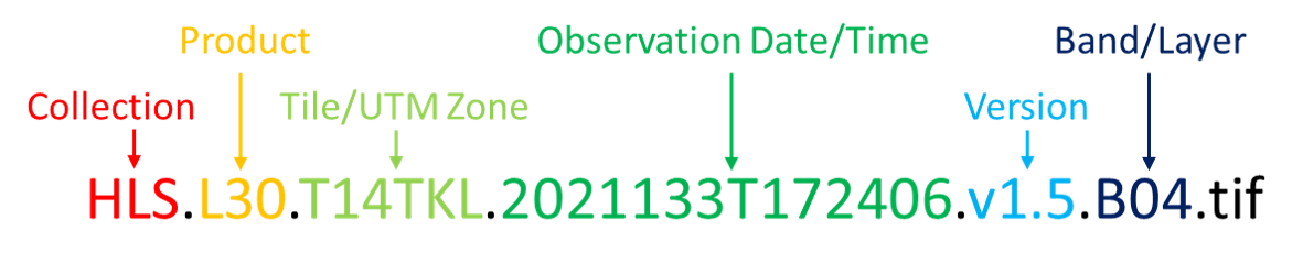
'https://data.lpdaac.earthdatacloud.nasa.gov/lp-prod-protected/HLSS30.020/HLS.S30.T14TKL.2021133T173859.v2.0/HLS.S30.T14TKL.2021133T173859.v2.0.B8A.tif']NOTE that HLS data is mapped to the Universal Transverse Mercator (UTM) projection and is tiled using the Sentinel-2 Military Grid Reference System (MGRS) UTM grid. Notice that in the list of links we have multiple tiles, i.e. T14TKL & T13TGF, that intersect with our region of interest. In this case, these two tiles represent neighboring UTM zones. The tiles can be discern from the file name, which is the last element in a link (far right) following the last forward slash (/) - e.g., HLS.L30.T14TKL.2021133T172406.v1.5.B04.tif. The figure below explains where to find the tile/UTM zone from the file name.
We will now split the list of links into separate logical sub-lists.
We have a list of links to data assets that meet our search and filtering criteria. Below we’ll split our list from above into lists first by tile/UTM zone and then further by individual bands bands. The commands that follow will do the splitting with python routines.
tile_dicts = defaultdict(list) # https://stackoverflow.com/questions/26367812/appending-to-list-in-python-dictionaryfor l in evi_band_links:
tile = l.split('.')[-6]
tile_dicts[tile].append(l)tile_dicts.keys()dict_keys(['T13TGF', 'T14TKL'])tile_dicts['T13TGF'][:5]['https://data.lpdaac.earthdatacloud.nasa.gov/lp-prod-protected/HLSL30.020/HLS.L30.T13TGF.2021133T172406.v2.0/HLS.L30.T13TGF.2021133T172406.v2.0.B04.tif',
'https://data.lpdaac.earthdatacloud.nasa.gov/lp-prod-protected/HLSL30.020/HLS.L30.T13TGF.2021133T172406.v2.0/HLS.L30.T13TGF.2021133T172406.v2.0.B05.tif',
'https://data.lpdaac.earthdatacloud.nasa.gov/lp-prod-protected/HLSL30.020/HLS.L30.T13TGF.2021133T172406.v2.0/HLS.L30.T13TGF.2021133T172406.v2.0.Fmask.tif',
'https://data.lpdaac.earthdatacloud.nasa.gov/lp-prod-protected/HLSL30.020/HLS.L30.T13TGF.2021133T172406.v2.0/HLS.L30.T13TGF.2021133T172406.v2.0.B02.tif',
'https://data.lpdaac.earthdatacloud.nasa.gov/lp-prod-protected/HLSS30.020/HLS.S30.T13TGF.2021133T173859.v2.0/HLS.S30.T13TGF.2021133T173859.v2.0.B8A.tif']Now we will create a separate list of data links for each tile
tile_links_T14TKL = tile_dicts['T14TKL']
tile_links_T13TGF = tile_dicts['T13TGF']# tile_links_T13TGF[:10]bands_dicts = defaultdict(list)for b in tile_links_T13TGF:
band = b.split('.')[-2]
bands_dicts[band].append(b)bands_dicts.keys()dict_keys(['B04', 'B05', 'Fmask', 'B02', 'B8A'])bands_dicts['B04']['https://data.lpdaac.earthdatacloud.nasa.gov/lp-prod-protected/HLSL30.020/HLS.L30.T13TGF.2021133T172406.v2.0/HLS.L30.T13TGF.2021133T172406.v2.0.B04.tif',
'https://data.lpdaac.earthdatacloud.nasa.gov/lp-prod-protected/HLSS30.020/HLS.S30.T13TGF.2021133T173859.v2.0/HLS.S30.T13TGF.2021133T173859.v2.0.B04.tif',
'https://data.lpdaac.earthdatacloud.nasa.gov/lp-prod-protected/HLSL30.020/HLS.L30.T13TGF.2021140T173021.v2.0/HLS.L30.T13TGF.2021140T173021.v2.0.B04.tif',
'https://data.lpdaac.earthdatacloud.nasa.gov/lp-prod-protected/HLSS30.020/HLS.S30.T13TGF.2021140T172859.v2.0/HLS.S30.T13TGF.2021140T172859.v2.0.B04.tif',
'https://data.lpdaac.earthdatacloud.nasa.gov/lp-prod-protected/HLSS30.020/HLS.S30.T13TGF.2021145T172901.v2.0/HLS.S30.T13TGF.2021145T172901.v2.0.B04.tif',
'https://data.lpdaac.earthdatacloud.nasa.gov/lp-prod-protected/HLSS30.020/HLS.S30.T13TGF.2021155T172901.v2.0/HLS.S30.T13TGF.2021155T172901.v2.0.B04.tif',
'https://data.lpdaac.earthdatacloud.nasa.gov/lp-prod-protected/HLSL30.020/HLS.L30.T13TGF.2021156T173029.v2.0/HLS.L30.T13TGF.2021156T173029.v2.0.B04.tif',
'https://data.lpdaac.earthdatacloud.nasa.gov/lp-prod-protected/HLSS30.020/HLS.S30.T13TGF.2021158T173901.v2.0/HLS.S30.T13TGF.2021158T173901.v2.0.B04.tif',
'https://data.lpdaac.earthdatacloud.nasa.gov/lp-prod-protected/HLSS30.020/HLS.S30.T13TGF.2021163T173909.v2.0/HLS.S30.T13TGF.2021163T173909.v2.0.B04.tif',
'https://data.lpdaac.earthdatacloud.nasa.gov/lp-prod-protected/HLSL30.020/HLS.L30.T13TGF.2021165T172422.v2.0/HLS.L30.T13TGF.2021165T172422.v2.0.B04.tif',
'https://data.lpdaac.earthdatacloud.nasa.gov/lp-prod-protected/HLSS30.020/HLS.S30.T13TGF.2021165T172901.v2.0/HLS.S30.T13TGF.2021165T172901.v2.0.B04.tif',
'https://data.lpdaac.earthdatacloud.nasa.gov/lp-prod-protected/HLSS30.020/HLS.S30.T13TGF.2021173T173909.v2.0/HLS.S30.T13TGF.2021173T173909.v2.0.B04.tif',
'https://data.lpdaac.earthdatacloud.nasa.gov/lp-prod-protected/HLSS30.020/HLS.S30.T13TGF.2021185T172901.v2.0/HLS.S30.T13TGF.2021185T172901.v2.0.B04.tif',
'https://data.lpdaac.earthdatacloud.nasa.gov/lp-prod-protected/HLSL30.020/HLS.L30.T13TGF.2021188T173037.v2.0/HLS.L30.T13TGF.2021188T173037.v2.0.B04.tif',
'https://data.lpdaac.earthdatacloud.nasa.gov/lp-prod-protected/HLSS30.020/HLS.S30.T13TGF.2021190T172859.v2.0/HLS.S30.T13TGF.2021190T172859.v2.0.B04.tif',
'https://data.lpdaac.earthdatacloud.nasa.gov/lp-prod-protected/HLSS30.020/HLS.S30.T13TGF.2021193T173909.v2.0/HLS.S30.T13TGF.2021193T173909.v2.0.B04.tif',
'https://data.lpdaac.earthdatacloud.nasa.gov/lp-prod-protected/HLSS30.020/HLS.S30.T13TGF.2021198T173911.v2.0/HLS.S30.T13TGF.2021198T173911.v2.0.B04.tif',
'https://data.lpdaac.earthdatacloud.nasa.gov/lp-prod-protected/HLSS30.020/HLS.S30.T13TGF.2021200T172859.v2.0/HLS.S30.T13TGF.2021200T172859.v2.0.B04.tif',
'https://data.lpdaac.earthdatacloud.nasa.gov/lp-prod-protected/HLSS30.020/HLS.S30.T13TGF.2021203T173909.v2.0/HLS.S30.T13TGF.2021203T173909.v2.0.B04.tif',
'https://data.lpdaac.earthdatacloud.nasa.gov/lp-prod-protected/HLSL30.020/HLS.L30.T13TGF.2021204T173042.v2.0/HLS.L30.T13TGF.2021204T173042.v2.0.B04.tif',
'https://data.lpdaac.earthdatacloud.nasa.gov/lp-prod-protected/HLSS30.020/HLS.S30.T13TGF.2021208T173911.v2.0/HLS.S30.T13TGF.2021208T173911.v2.0.B04.tif',
'https://data.lpdaac.earthdatacloud.nasa.gov/lp-prod-protected/HLSS30.020/HLS.S30.T13TGF.2021210T172859.v2.0/HLS.S30.T13TGF.2021210T172859.v2.0.B04.tif',
'https://data.lpdaac.earthdatacloud.nasa.gov/lp-prod-protected/HLSS30.020/HLS.S30.T13TGF.2021215T172901.v2.0/HLS.S30.T13TGF.2021215T172901.v2.0.B04.tif',
'https://data.lpdaac.earthdatacloud.nasa.gov/lp-prod-protected/HLSS30.020/HLS.S30.T13TGF.2021218T173911.v2.0/HLS.S30.T13TGF.2021218T173911.v2.0.B04.tif',
'https://data.lpdaac.earthdatacloud.nasa.gov/lp-prod-protected/HLSL30.020/HLS.L30.T13TGF.2021220T173049.v2.0/HLS.L30.T13TGF.2021220T173049.v2.0.B04.tif',
'https://data.lpdaac.earthdatacloud.nasa.gov/lp-prod-protected/HLSS30.020/HLS.S30.T13TGF.2021220T172859.v2.0/HLS.S30.T13TGF.2021220T172859.v2.0.B04.tif',
'https://data.lpdaac.earthdatacloud.nasa.gov/lp-prod-protected/HLSS30.020/HLS.S30.T13TGF.2021223T173909.v2.0/HLS.S30.T13TGF.2021223T173909.v2.0.B04.tif',
'https://data.lpdaac.earthdatacloud.nasa.gov/lp-prod-protected/HLSS30.020/HLS.S30.T13TGF.2021228T173911.v2.0/HLS.S30.T13TGF.2021228T173911.v2.0.B04.tif',
'https://data.lpdaac.earthdatacloud.nasa.gov/lp-prod-protected/HLSL30.020/HLS.L30.T13TGF.2021229T172441.v2.0/HLS.L30.T13TGF.2021229T172441.v2.0.B04.tif',
'https://data.lpdaac.earthdatacloud.nasa.gov/lp-prod-protected/HLSS30.020/HLS.S30.T13TGF.2021230T172859.v2.0/HLS.S30.T13TGF.2021230T172859.v2.0.B04.tif',
'https://data.lpdaac.earthdatacloud.nasa.gov/lp-prod-protected/HLSS30.020/HLS.S30.T13TGF.2021235T172901.v2.0/HLS.S30.T13TGF.2021235T172901.v2.0.B04.tif',
'https://data.lpdaac.earthdatacloud.nasa.gov/lp-prod-protected/HLSS30.020/HLS.S30.T13TGF.2021243T173859.v2.0/HLS.S30.T13TGF.2021243T173859.v2.0.B04.tif']To complete this exercise, we will save the individual link lists as separate text files with descriptive names.
NOTE: If you are running the notebook from the tutorials-templates directory, please use the following path to write to the data directory: “../tutorials/data/{name}”
for k, v in bands_dicts.items():
    name = (f'HTTPS_T13TGF_{k}_Links.txt')
    with open(f'./data/{name}', 'w') as f:    # use ../tutorials/data/{name} as your path if running the notebook from "tutorials-template"
        for l in v:
f.write(f"{l}" + '\n')for k, v in bands_dicts.items():
name = (f'S3_T13TGF_{k}_Links.txt')
with open(f'./data/{name}', 'w') as f: # use ../tutorials/data/{name} as your path if running the notebook from "tutorials-template"
for l in v:
s3l = l.replace('https://data.lpdaac.earthdatacloud.nasa.gov/', 's3://')
f.write(f"{s3l}" + '\n')