03. Introduction to `xarray`

Why do we need `xarray`?

As Geoscientists, we often work with time series of data with two or more dimensions: a time series of calibrated, orthorectified satellite images; two-dimensional grids of surface air temperature from an atmospheric reanalysis; or three-dimensional (level, x, y) cubes of ocean salinity from an ocean model. These data are often provided in GeoTIFF, NetCDF or HDF format with rich and useful metadata that we want to retain, or even use in our analysis. Common analyses include calculating means, standard deviations and anomalies over time or one or more spatial dimensions (e.g. zonal means). Model output often includes multiple variables that you want to apply similar analyses to.

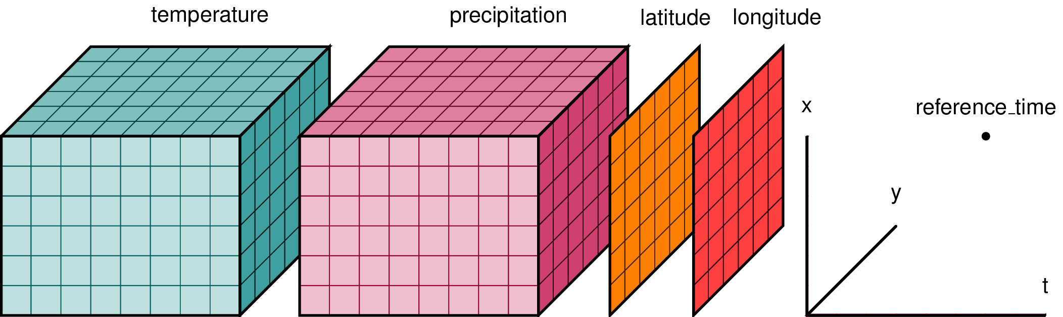
The schematic above shows a typical data structure for multi-dimensional data. There are two data cubes, one for temperature and one for precipitation. Common coordinate variables, in this case latitude, longitude and time are associated with each variable. Each variable, including coordinate variables, will have a set of attributes: name, units, missing value, etc. The file containing the data may also have attributes: source of the data, model name coordinate reference system if the data are projected. Writing code using low-level packages such as netcdf4 and numpy to read the data, then perform analysis, and write the results to file is time consuming and prone to errors.

What is `xarray`

xarray is an open-source project and python package to work with labelled multi-dimensional arrays. It is leverages numpy, pandas, matplotlib and dask to build Dataset and DataArray objects with built-in methods to subset, analyze, interpolate, and plot multi-dimensional data. It makes working with multi-dimensional data cubes efficient and fun. It will change your life for the better. You’ll be more attractive, more interesting, and better equiped to take on lifes challenges.

What you will learn from this tutorial

In this tutorial you will learn how to:

load a netcdf file into xarray
interrogate the Dataset and understand the difference between DataArray and Dataset
subset a Dataset
calculate annual and monthly mean fields
calculate a time series of zonal means
plot these results

As always, we’ll start by importing xarray. We’ll follow convention by giving the module the shortname xr

import xarray as xr
xr.set_options(keep_attrs=True)

I’m going to use one of xarray’s tutorial datasets. In this case, air temperature from the NCEP reanalysis. I’ll assign the result of the open_dataset to ds. I may change this to access a dataset directly

ds = xr.tutorial.open_dataset("air_temperature")

As we are in an interactive environment, we can just type ds to see what we have.

ds

First thing to notice is that ds is an xarray.Dataset object. It has dimensions, lat, lon, and time. It also has coordinate variables with the same names as these dimensions. These coordinate variables are 1-dimensional. This is a NetCDF convention. The Dataset contains one data variable, air. This has dimensions (time, lat, lon).

Clicking on the document icon reveals attributes for each variable. Clicking on the disk icon reveals a representation of the data.

Each of the data and coordinate variables can be accessed and examined using the variable name as a key.

ds.air

ds['air']

These are xarray.DataArray objects. This is the basic building block for xarray.

Variables can also be accessed as attributes of ds.

ds.time

A major difference between accessing a variable as an attribute versus using a key is that the attribute is read-only but the key method can be used to update the variable. For example, if I want to convert the units of air from Kelvin to degrees Celsius.

ds['air'] = ds.air - 273.15

This approach can also be used to add new variables

ds['air_kelvin'] = ds.air + 273.15

It is helpful to update attributes such as units, this saves time, confusion and mistakes, especially when you save the dataset.

ds['air'].attrs['units'] = 'degC'

ds

Subsetting and Indexing

Subsetting and indexing methods depend on whether you are working with a Dataset or DataArray. A DataArray can be accessed using positional indexing just like a numpy array. To access the temperature field for the first time step, you do the following.

ds['air'][0,:,:]

Note this returns a DataArray with coordinates but not attributes.

However, the real power is being able to access variables using coordinate variables. I can get the same subset using the following. (It’s also more explicit about what is being selected and robust in case I modify the DataArray and expect the same output.)

ds['air'].sel(time='2013-01-01').time

ds.air.sel(time='2013-01-01')

I can also do slices. I’ll extract temperatures for the state of Colorado. The bounding box for the state is [-109 E, -102 E, 37 N, 41 N].

In the code below, pay attention to both the order of the coordinates and the range of values. The first value of the lat coordinate variable is 41 N, the second value is 37 N. Unfortunately, xarray expects slices of coordinates to be in the same order as the coordinates. Note lon is 0 to 360 not -180 to 180, and I let python calculate it for me within the slice.

ds.air.sel(lat=slice(41.,37.), lon=slice(360-109,360-102))

What if we want temperature for a point, for example Denver, CO (39.72510678889283 N, -104.98785545855408 E). xarray can handle this! If we just want data from the nearest grid point, we can use sel and specify the method as “nearest”.

denver_lat, denver_lon = 39.72510678889283, -104.98785545855408

ds.air.sel(lat=denver_lat, lon=360+denver_lon, method='nearest')

If we want to interpolate, we can use interp(). In this case I use linear or bilinear interpolation.

interp() can also be used to resample data to a new grid and even reproject data

ds.air.interp(lat=denver_lat, lon=360+denver_lon, method='linear')

sel() and interp() can also be used on Dataset objects.

ds.sel(lat=slice(41.,37.), lon=slice(360-109,360-102))

ds.interp(lat=denver_lat, lon=360+denver_lon, method='linear')

Analysis

As a simple example, let’s try to calculate a mean field for the whole time range.

ds.mean(dim='time')

We can also calculate a zonal mean (averaging over longitude)

ds.mean(dim='lon')

Other aggregation methods include min(), max(), std(), along with others.

ds.std(dim='time')

The data we have are in 6h timesteps. This can be resampled to daily or monthly. If you are familiar with pandas, xarray uses the same methods.

ds.resample(time='M').mean()

ds_mon = ds.resample(time='M').mean()
ds_mon

This is a really short time series but as an example, let’s calculate a monthly climatology (at least for 2 months). For this we can use groupby()

ds_clim = ds_mon.groupby(ds_mon.time.dt.month).mean()

Plot results

Finally, let’s plot the results! This will plot the lat/lon axes of the original ds DataArray.

ds_clim.air.sel(month=10).plot()

Why do we need xarray?

What is xarray