Analyzing Sea Level Rise with NASA Earthdata

image.png

Overview

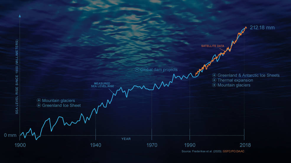
This tutorial analyzes global sea level rise from satellite altimetry data and compares it to a historic record. We will be reproducing the plot from this infographic: NASA-led Study Reveals the Causes of Sea Level Rise Since 1900.

Learning Objectives

• Search for data programmatically using keywords
• Access data within the AWS cloud using the earthaccess python library
• Visualize sea level rise trends from altimetry datasets and compare against historic records

Requirements

1. Compute environment - This notebook can only be run in an AWS Cloud instance running in the us-west-2 region.

2. Earthdata Login

An Earthdata Login account is required to access data, as well as discover restricted data, from the NASA Earthdata system. Thus, to access NASA data, you need Earthdata Login. Please visit https://urs.earthdata.nasa.gov to register and manage your Earthdata Login account. This account is free to create and only takes a moment to set up.

Install Packages

import earthaccess
import xarray as xr
from pyproj import Geod
import numpy as np
import hvplot.xarray
from matplotlib import pyplot as plt
from pprint import pprint

We recommend authenticating your Earthdata Login (EDL) information using the earthaccess python package as follows:

auth = earthaccess.login(strategy="netrc") # works if the EDL login already been persisted to a netrc
if not auth.authenticated:
    # ask for EDL credentials and persist them in a .netrc file
    auth = earthaccess.login(strategy="interactive", persist=True)

You're now authenticated with NASA Earthdata Login
Using token with expiration date: 09/10/2023
Using .netrc file for EDL

Search for Sea Surface Height Data

Let’s find the first four collections that match a keyword search for Sea Surface Height and print out the first two.

collections = earthaccess.collection_query().keyword("SEA SURFACE HEIGHT").cloud_hosted(True).get(4)

# Let's print 2 collections
for collection in collections[0:2]:
    # pprint(collection.summary())
    print(pprint(collection.summary()), collection.abstract(), "\n", collection["umm"]["DOI"], "\n\n")

{'cloud-info': {'Region': 'us-west-2',
                'S3BucketAndObjectPrefixNames': ['podaac-ops-cumulus-public/SEA_SURFACE_HEIGHT_ALT_GRIDS_L4_2SATS_5DAY_6THDEG_V_JPL2205/',
                                                 'podaac-ops-cumulus-protected/SEA_SURFACE_HEIGHT_ALT_GRIDS_L4_2SATS_5DAY_6THDEG_V_JPL2205/'],
                'S3CredentialsAPIDocumentationURL': 'https://archive.podaac.earthdata.nasa.gov/s3credentialsREADME',
                'S3CredentialsAPIEndpoint': 'https://archive.podaac.earthdata.nasa.gov/s3credentials'},
 'concept-id': 'C2270392799-POCLOUD',
 'file-type': "[{'Format': 'netCDF-4', 'FormatType': 'Native', "
              "'AverageFileSize': 9.7, 'AverageFileSizeUnit': 'MB'}]",
 'get-data': ['https://cmr.earthdata.nasa.gov/virtual-directory/collections/C2270392799-POCLOUD',
              'https://search.earthdata.nasa.gov/search/granules?p=C2270392799-POCLOUD'],
 'short-name': 'SEA_SURFACE_HEIGHT_ALT_GRIDS_L4_2SATS_5DAY_6THDEG_V_JPL2205',
 'version': '2205'}
None This dataset provides gridded Sea Surface Height Anomalies (SSHA) above a mean sea surface, on a 1/6th degree grid every 5 days. It contains the fully corrected heights, with a delay of up to 3 months. The gridded data are derived from the along-track SSHA data of TOPEX/Poseidon, Jason-1, Jason-2, Jason-3 and Jason-CS (Sentinel-6) as reference data from the level 2 along-track data found at https://podaac.jpl.nasa.gov/dataset/MERGED_TP_J1_OSTM_OST_CYCLES_V51, plus ERS-1, ERS-2, Envisat, SARAL-AltiKa, CryoSat-2, Sentinel-3A, Sentinel-3B, depending on the date, from the RADS database. The date given in the grid files is the center of the 5-day window. The grids were produced from altimeter data using Kriging interpolation, which gives best linear prediction based upon prior knowledge of covariance. 
 {'DOI': '10.5067/SLREF-CDRV3', 'Authority': 'https://doi.org'} 


{'cloud-info': {'Region': 'us-west-2',
                'S3BucketAndObjectPrefixNames': ['nsidc-cumulus-prod-protected/ATLAS/ATL21/003',
                                                 'nsidc-cumulus-prod-public/ATLAS/ATL21/003'],
                'S3CredentialsAPIDocumentationURL': 'https://data.nsidc.earthdatacloud.nasa.gov/s3credentialsREADME',
                'S3CredentialsAPIEndpoint': 'https://data.nsidc.earthdatacloud.nasa.gov/s3credentials'},
 'concept-id': 'C2753316241-NSIDC_CPRD',
 'file-type': "[{'FormatType': 'Native', 'Format': 'HDF5', "
              "'FormatDescription': 'HTTPS'}]",
 'get-data': ['https://search.earthdata.nasa.gov/search?q=ATL21+V003'],
 'short-name': 'ATL21',
 'version': '003'}
None This data set contains daily and monthly gridded polar sea surface height (SSH) anomalies, derived from the along-track ATLAS/ICESat-2 L3A Sea Ice Height product (ATL10, V6). The ATL10 product identifies leads in sea ice and establishes a reference sea surface used to estimate SSH in 10 km along-track segments. ATL21 aggregates the ATL10 along-track SSH estimates and computes daily and monthly gridded SSH anomaly in NSIDC Polar Stereographic Northern and Southern Hemisphere 25 km grids. 
 {'DOI': '10.5067/ATLAS/ATL21.003'} 

Access Data

The first dataset looks like it contains data from many altimetry missions, let’s explore a bit more! We will access the first granule of the SEA_SURFACE_HEIGHT_ALT_GRIDS_L4_2SATS_5DAY_6THDEG_V_JPL2205 collection in the month of May for every year that data is available and open the granules via xarray.

granules = []
for year in range(1990, 2019):
    granule = earthaccess.granule_query().short_name("SEA_SURFACE_HEIGHT_ALT_GRIDS_L4_2SATS_5DAY_6THDEG_V_JPL2205").temporal(f"{year}-05", f"{year}-06").get(1)
    if len(granule)>0:
        granules.append(granule[0])
print(f"Total granules: {len(granules)}")       

Total granules: 26

%%time

ds_SSH = xr.open_mfdataset(earthaccess.open(granules), chunks={})
ds_SSH

 Opening 26 granules, approx size: 0.0 GB
CPU times: user 5.79 s, sys: 846 ms, total: 6.64 s
Wall time: 24.9 s

<xarray.Dataset>
Dimensions:      (Time: 26, Longitude: 2160, nv: 2, Latitude: 960)
Coordinates:
  * Longitude    (Longitude) float32 0.08333 0.25 0.4167 ... 359.6 359.8 359.9
  * Latitude     (Latitude) float32 -79.92 -79.75 -79.58 ... 79.58 79.75 79.92
  * Time         (Time) datetime64[ns] 1993-05-03T12:00:00 ... 2018-05-02T12:...
Dimensions without coordinates: nv
Data variables:
    Lon_bounds   (Time, Longitude, nv) float32 dask.array<chunksize=(1, 2160, 2), meta=np.ndarray>
    Lat_bounds   (Time, Latitude, nv) float32 dask.array<chunksize=(1, 960, 2), meta=np.ndarray>
    Time_bounds  (Time, nv) datetime64[ns] dask.array<chunksize=(1, 2), meta=np.ndarray>
    SLA          (Time, Latitude, Longitude) float32 dask.array<chunksize=(1, 960, 2160), meta=np.ndarray>
    SLA_ERR      (Time, Latitude, Longitude) float32 dask.array<chunksize=(1, 960, 2160), meta=np.ndarray>
Attributes: (12/21)
    Conventions:            CF-1.6
    ncei_template_version:  NCEI_NetCDF_Grid_Template_v2.0
    Institution:            Jet Propulsion Laboratory
    geospatial_lat_min:     -79.916664
    geospatial_lat_max:     79.916664
    geospatial_lon_min:     0.083333336
    ...                     ...
    version_number:         2205
    Data_Pnts_Each_Sat:     {"16": 780190, "1001": 668288}
    source_version:         commit dc95db885c920084614a41849ce5a7d417198ef3
    SLA_Global_MEAN:        -0.027657876081274502
    SLA_Global_STD:         0.0859016072308609
    latency:                final

xarray.Dataset

• Dimensions:
  • Time: 26
  • Longitude: 2160
  • nv: 2
  • Latitude: 960
• Coordinates: (3)
  • Longitude
    (Longitude)
    float32
    0.08333 0.25 0.4167 ... 359.8 359.9

    standard_name :

    longitude

    units :

    degrees_east

    point_spacing :

    even

    long_name :

    longitude

    axis :

    X

    bounds :

    Lon_bounds

    array([8.333334e-02, 2.500000e-01, 4.166667e-01, ..., 3.595833e+02,
           3.597500e+02, 3.599167e+02], dtype=float32)

  • Latitude
    (Latitude)
    float32
    -79.92 -79.75 ... 79.75 79.92

    standard_name :

    latitude

    units :

    degrees_north

    point_spacing :

    even

    long_name :

    latitude

    axis :

    Y

    bounds :

    Lat_bounds

    array([-79.916664, -79.75    , -79.583336, ...,  79.583336,  79.75    ,
            79.916664], dtype=float32)

  • Time
    (Time)
    datetime64[ns]
    1993-05-03T12:00:00 ... 2018-05-...

    standard_name :

    time

    long_name :

    Time

    bounds :

    Time_bounds

    axis :

    T

    array(['1993-05-03T12:00:00.000000000', '1994-05-03T12:00:00.000000000',
           '1995-05-03T12:00:00.000000000', '1996-05-02T12:00:00.000000000',
           '1997-05-02T12:00:00.000000000', '1998-05-02T12:00:00.000000000',
           '1999-05-02T12:00:00.000000000', '2000-05-01T12:00:00.000000000',
           '2001-05-01T12:00:00.000000000', '2002-05-01T12:00:00.000000000',
           '2003-05-01T12:00:00.000000000', '2004-05-05T12:00:00.000000000',
           '2005-05-05T12:00:00.000000000', '2006-05-05T12:00:00.000000000',
           '2007-05-05T12:00:00.000000000', '2008-05-04T12:00:00.000000000',
           '2009-05-04T12:00:00.000000000', '2010-05-04T12:00:00.000000000',
           '2011-05-04T12:00:00.000000000', '2012-05-03T12:00:00.000000000',
           '2013-05-03T12:00:00.000000000', '2014-05-03T12:00:00.000000000',
           '2015-05-03T12:00:00.000000000', '2016-05-02T12:00:00.000000000',
           '2017-05-02T12:00:00.000000000', '2018-05-02T12:00:00.000000000'],
          dtype='datetime64[ns]')

• Data variables: (5)
  • Lon_bounds
    (Time, Longitude, nv)
    float32
    dask.array<chunksize=(1, 2160, 2), meta=np.ndarray>

    units :

    degrees_east

    comment :

    longitude values at the west and east bounds of each pixel.

    Array Chunk Bytes 438.75 kiB 16.88 kiB Shape (26, 2160, 2) (1, 2160, 2) Dask graph 26 chunks in 79 graph layers Data type float32 numpy.ndarray

    Lat_bounds

    (Time, Latitude, nv)

    float32

    dask.array<chunksize=(1, 960, 2), meta=np.ndarray>

    

    units :

    degrees_north

    comment :

    latitude values at the north and south bounds of each pixel.

    Array Chunk Bytes 195.00 kiB 7.50 kiB Shape (26, 960, 2) (1, 960, 2) Dask graph 26 chunks in 79 graph layers Data type float32 numpy.ndarray

    Time_bounds

    (Time, nv)

    datetime64[ns]

    dask.array<chunksize=(1, 2), meta=np.ndarray>

    

    comment :

    Time bounds for each time value, same value as time variable. The time variable is defined on points instead of on bounding boxes.

    Array Chunk Bytes 416 B 16 B Shape (26, 2) (1, 2) Dask graph 26 chunks in 53 graph layers Data type datetime64[ns] numpy.ndarray

    SLA

    (Time, Latitude, Longitude)

    float32

    dask.array<chunksize=(1, 960, 2160), meta=np.ndarray>

    

    units :

    m

    long_name :

    Sea Level Anomaly Estimate

    standard_name :

    sea_surface_height_above_sea_level

    alias :

    sea_surface_height_above_sea_level

    Array Chunk Bytes 205.66 MiB 7.91 MiB Shape (26, 960, 2160) (1, 960, 2160) Dask graph 26 chunks in 53 graph layers Data type float32 numpy.ndarray

    SLA_ERR

    (Time, Latitude, Longitude)

    float32

    dask.array<chunksize=(1, 960, 2160), meta=np.ndarray>

    

    units :

    m

    long_name :

    Sea Level Anomaly Error Estimate

    Array Chunk Bytes 205.66 MiB 7.91 MiB Shape (26, 960, 2160) (1, 960, 2160) Dask graph 26 chunks in 53 graph layers Data type float32 numpy.ndarray

• Indexes: (3)
  • Longitude
    PandasIndex

    PandasIndex(Index([0.0833333358168602,               0.25, 0.4166666567325592,
           0.5833333134651184,               0.75, 0.9166666865348816,
           1.0833333730697632,               1.25, 1.4166666269302368,
           1.5833333730697632,
           ...
            358.4166564941406,  358.5833435058594,             358.75,
            358.9166564941406,  359.0833435058594,             359.25,
            359.4166564941406,  359.5833435058594,             359.75,
            359.9166564941406],
          dtype='float32', name='Longitude', length=2160))

  • Latitude
    PandasIndex

    PandasIndex(Index([-79.91666412353516,             -79.75, -79.58333587646484,
           -79.41666412353516,             -79.25, -79.08333587646484,
           -78.91666412353516,             -78.75, -78.58333587646484,
           -78.41666412353516,
           ...
            78.41666412353516,  78.58333587646484,              78.75,
            78.91666412353516,  79.08333587646484,              79.25,
            79.41666412353516,  79.58333587646484,              79.75,
            79.91666412353516],
          dtype='float32', name='Latitude', length=960))

  • Time
    PandasIndex

    PandasIndex(DatetimeIndex(['1993-05-03 12:00:00', '1994-05-03 12:00:00',
                   '1995-05-03 12:00:00', '1996-05-02 12:00:00',
                   '1997-05-02 12:00:00', '1998-05-02 12:00:00',
                   '1999-05-02 12:00:00', '2000-05-01 12:00:00',
                   '2001-05-01 12:00:00', '2002-05-01 12:00:00',
                   '2003-05-01 12:00:00', '2004-05-05 12:00:00',
                   '2005-05-05 12:00:00', '2006-05-05 12:00:00',
                   '2007-05-05 12:00:00', '2008-05-04 12:00:00',
                   '2009-05-04 12:00:00', '2010-05-04 12:00:00',
                   '2011-05-04 12:00:00', '2012-05-03 12:00:00',
                   '2013-05-03 12:00:00', '2014-05-03 12:00:00',
                   '2015-05-03 12:00:00', '2016-05-02 12:00:00',
                   '2017-05-02 12:00:00', '2018-05-02 12:00:00'],
                  dtype='datetime64[ns]', name='Time', freq=None))

• Attributes: (21)

  Conventions :

  CF-1.6

  ncei_template_version :

  NCEI_NetCDF_Grid_Template_v2.0

  Institution :

  Jet Propulsion Laboratory

  geospatial_lat_min :

  -79.916664

  geospatial_lat_max :

  79.916664

  geospatial_lon_min :

  0.083333336

  geospatial_lon_max :

  359.91666

  time_coverage_start :

  1993-05-03

  time_coverage_end :

  1993-05-03

  date_created :

  2022-10-30T20:40:50.716092

  title :

  Sea Level Anomaly Estimate based on Altimeter Data, final product (replaced interim version).

  short_name :

  SEA_SURFACE_HEIGHT_ALT_GRIDS_L4_2SATS_5DAY_6THDEG_V_JPL2205

  long_name :

  MEaSUREs Gridded Sea Surface Height Anomalies Version 2205

  summary :

  Sea level anomaly grids from altimeter data using Kriging interpolation, which gives best linear prediction based upon prior knowledge of covariance.

  DOI :

  10.5067/SLREF-CDRV3

  version_number :

  2205

  Data_Pnts_Each_Sat :

  {"16": 780190, "1001": 668288}

  source_version :

  commit dc95db885c920084614a41849ce5a7d417198ef3

  SLA_Global_MEAN :

  -0.027657876081274502

  SLA_Global_STD :

  0.0859016072308609

  latency :

  final

Plot Sea Level Anomalies

ds_SSH.SLA.hvplot.image(y='Latitude', x='Longitude', cmap='viridis')

Recreate the Sea Level Rise Infographic

First, we define a function that will calculate the area in 1/6 by 1/6 degree boxes in order to calculate the global mean of the SSH later.

def ssl_area(lats):
    """
    Calculate the area associated with a 1/6 by 1/6 degree box at latitude specified in 'lats'.
    
    Parameter
    ==========
    lats: a list or numpy array of size N the latitudes of interest. 
    
    Return
    =======
    out: Array (N) area values (unit: m^2)
    """
    # Define WGS84 as CRS:
    geod = Geod(ellps='WGS84')
    dx=1/12.0
    # create a lambda function for calculating the perimeters of the boxes
    c_area=lambda lat: geod.polygon_area_perimeter(np.r_[-dx,dx,dx,-dx], lat+np.r_[-dx,-dx,dx,dx])[0]
    out=[]
    for lat in lats:
        out.append(c_area(lat))
    return np.array(out)

Let’s use the function on our Sea Surface Height dataset.

# note: they rotated the data in the last release, this operation used to be (1,-1)
ssh_area = ssl_area(ds_SSH.Latitude.data).reshape(-1,1)
print(ssh_area.shape)

(960, 1)

Next, we find and open the historic record dataset also using earthaccess and xarray.

historic_ts_results = earthaccess.search_data(short_name='JPL_RECON_GMSL')

Granules found: 1

historic_ts=xr.open_mfdataset(earthaccess.open([historic_ts_results[0]]), engine='h5netcdf')
historic_ts

 Opening 1 granules, approx size: 0.0 GB

<xarray.Dataset>
Dimensions:                                             (time: 119)
Coordinates:
  * time                                                (time) datetime64[ns] ...
Data variables: (12/21)
    global_average_sea_level_change                     (time) float32 dask.array<chunksize=(119,), meta=np.ndarray>
    global_average_sea_level_change_upper               (time) float32 dask.array<chunksize=(119,), meta=np.ndarray>
    global_average_sea_level_change_lower               (time) float32 dask.array<chunksize=(119,), meta=np.ndarray>
    glac_mean                                           (time) float32 dask.array<chunksize=(119,), meta=np.ndarray>
    glac_upper                                          (time) float32 dask.array<chunksize=(119,), meta=np.ndarray>
    glac_lower                                          (time) float32 dask.array<chunksize=(119,), meta=np.ndarray>
    ...                                                  ...
    global_average_thermosteric_sea_level_change        (time) float32 dask.array<chunksize=(119,), meta=np.ndarray>
    global_average_thermosteric_sea_level_change_upper  (time) float32 dask.array<chunksize=(119,), meta=np.ndarray>
    global_average_thermosteric_sea_level_change_lower  (time) float32 dask.array<chunksize=(119,), meta=np.ndarray>
    sum_of_contrib_processes_mean                       (time) float32 dask.array<chunksize=(119,), meta=np.ndarray>
    sum_of_contrib_processes_upper                      (time) float32 dask.array<chunksize=(119,), meta=np.ndarray>
    sum_of_contrib_processes_lower                      (time) float32 dask.array<chunksize=(119,), meta=np.ndarray>
Attributes: (12/42)
    title:                     Global sea-level changes and contributing proc...
    summary:                   This file contains reconstructed global-mean s...
    id:                        10.5067/GMSLT-FJPL1
    naming_authority:          gov.nasa.jpl
    source:                    Frederikse et al. The causes of sea-level rise...
    project:                   NASA sea-level change science team (N-SLCT)
    ...                        ...
    time_coverage_start:       1900-01-01
    time_coverage_end:         2018-12-31
    time_coverage_duration:    P119Y
    time_coverage_resolution:  P1Y
    date_created:              2020-07-28
    date_modified:             2020-09-14

xarray.Dataset

• Dimensions:
  • time: 119
• Coordinates: (1)
  • time
    (time)
    datetime64[ns]
    1900-06-15 ... 2018-06-15

    long_name :

    time

    standard_name :

    time

    array(['1900-06-15T00:00:00.000000000', '1901-06-15T00:00:00.000000000',
           '1902-06-15T00:00:00.000000000', '1903-06-15T00:00:00.000000000',
           '1904-06-15T00:00:00.000000000', '1905-06-15T00:00:00.000000000',
           '1906-06-15T00:00:00.000000000', '1907-06-15T00:00:00.000000000',
           '1908-06-15T00:00:00.000000000', '1909-06-15T00:00:00.000000000',
           '1910-06-15T00:00:00.000000000', '1911-06-15T00:00:00.000000000',
           '1912-06-15T00:00:00.000000000', '1913-06-15T00:00:00.000000000',
           '1914-06-15T00:00:00.000000000', '1915-06-15T00:00:00.000000000',
           '1916-06-15T00:00:00.000000000', '1917-06-15T00:00:00.000000000',
           '1918-06-15T00:00:00.000000000', '1919-06-15T00:00:00.000000000',
           '1920-06-15T00:00:00.000000000', '1921-06-15T00:00:00.000000000',
           '1922-06-15T00:00:00.000000000', '1923-06-15T00:00:00.000000000',
           '1924-06-15T00:00:00.000000000', '1925-06-15T00:00:00.000000000',
           '1926-06-15T00:00:00.000000000', '1927-06-15T00:00:00.000000000',
           '1928-06-15T00:00:00.000000000', '1929-06-15T00:00:00.000000000',
           '1930-06-15T00:00:00.000000000', '1931-06-15T00:00:00.000000000',
           '1932-06-15T00:00:00.000000000', '1933-06-15T00:00:00.000000000',
           '1934-06-15T00:00:00.000000000', '1935-06-15T00:00:00.000000000',
           '1936-06-15T00:00:00.000000000', '1937-06-15T00:00:00.000000000',
           '1938-06-15T00:00:00.000000000', '1939-06-15T00:00:00.000000000',
           '1940-06-15T00:00:00.000000000', '1941-06-15T00:00:00.000000000',
           '1942-06-15T00:00:00.000000000', '1943-06-15T00:00:00.000000000',
           '1944-06-15T00:00:00.000000000', '1945-06-15T00:00:00.000000000',
           '1946-06-15T00:00:00.000000000', '1947-06-15T00:00:00.000000000',
           '1948-06-15T00:00:00.000000000', '1949-06-15T00:00:00.000000000',
           '1950-06-15T00:00:00.000000000', '1951-06-15T00:00:00.000000000',
           '1952-06-15T00:00:00.000000000', '1953-06-15T00:00:00.000000000',
           '1954-06-15T00:00:00.000000000', '1955-06-15T00:00:00.000000000',
           '1956-06-15T00:00:00.000000000', '1957-06-15T00:00:00.000000000',
           '1958-06-15T00:00:00.000000000', '1959-06-15T00:00:00.000000000',
           '1960-06-15T00:00:00.000000000', '1961-06-15T00:00:00.000000000',
           '1962-06-15T00:00:00.000000000', '1963-06-15T00:00:00.000000000',
           '1964-06-15T00:00:00.000000000', '1965-06-15T00:00:00.000000000',
           '1966-06-15T00:00:00.000000000', '1967-06-15T00:00:00.000000000',
           '1968-06-15T00:00:00.000000000', '1969-06-15T00:00:00.000000000',
           '1970-06-15T00:00:00.000000000', '1971-06-15T00:00:00.000000000',
           '1972-06-15T00:00:00.000000000', '1973-06-15T00:00:00.000000000',
           '1974-06-15T00:00:00.000000000', '1975-06-15T00:00:00.000000000',
           '1976-06-15T00:00:00.000000000', '1977-06-15T00:00:00.000000000',
           '1978-06-15T00:00:00.000000000', '1979-06-15T00:00:00.000000000',
           '1980-06-15T00:00:00.000000000', '1981-06-15T00:00:00.000000000',
           '1982-06-15T00:00:00.000000000', '1983-06-15T00:00:00.000000000',
           '1984-06-15T00:00:00.000000000', '1985-06-15T00:00:00.000000000',
           '1986-06-15T00:00:00.000000000', '1987-06-15T00:00:00.000000000',
           '1988-06-15T00:00:00.000000000', '1989-06-15T00:00:00.000000000',
           '1990-06-15T00:00:00.000000000', '1991-06-15T00:00:00.000000000',
           '1992-06-15T00:00:00.000000000', '1993-06-15T00:00:00.000000000',
           '1994-06-15T00:00:00.000000000', '1995-06-15T00:00:00.000000000',
           '1996-06-15T00:00:00.000000000', '1997-06-15T00:00:00.000000000',
           '1998-06-15T00:00:00.000000000', '1999-06-15T00:00:00.000000000',
           '2000-06-15T00:00:00.000000000', '2001-06-15T00:00:00.000000000',
           '2002-06-15T00:00:00.000000000', '2003-06-15T00:00:00.000000000',
           '2004-06-15T00:00:00.000000000', '2005-06-15T00:00:00.000000000',
           '2006-06-15T00:00:00.000000000', '2007-06-15T00:00:00.000000000',
           '2008-06-15T00:00:00.000000000', '2009-06-15T00:00:00.000000000',
           '2010-06-15T00:00:00.000000000', '2011-06-15T00:00:00.000000000',
           '2012-06-15T00:00:00.000000000', '2013-06-15T00:00:00.000000000',
           '2014-06-15T00:00:00.000000000', '2015-06-15T00:00:00.000000000',
           '2016-06-15T00:00:00.000000000', '2017-06-15T00:00:00.000000000',
           '2018-06-15T00:00:00.000000000'], dtype='datetime64[ns]')

• Data variables: (21)
  • global_average_sea_level_change
    (time)
    float32
    dask.array<chunksize=(119,), meta=np.ndarray>

    units :

    mm

    long_name :

    Observed global-average sea level (mean value)

    valid_min :

    -1000000.0

    valid_max :

    1000000.0

    comment :

    Value is relative to 2002-2019 baseline

    standard_name :

    global_average_sea_level_change

    coverage_content_type :

    physicalMeasurement

    Array Chunk Bytes 476 B 476 B Shape (119,) (119,) Dask graph 1 chunks in 2 graph layers Data type float32 numpy.ndarray

    global_average_sea_level_change_upper

    (time)

    float32

    dask.array<chunksize=(119,), meta=np.ndarray>

    

    units :

    mm

    long_name :

    Observed global-average sea level (upper bound)

    standard_name :

    global_average_sea_level_change

    valid_min :

    -1000000.0

    valid_max :

    1000000.0

    comment :

    Value is relative to 2002-2019 baseline

    coverage_content_type :

    physicalMeasurement

    Array Chunk Bytes 476 B 476 B Shape (119,) (119,) Dask graph 1 chunks in 2 graph layers Data type float32 numpy.ndarray

    global_average_sea_level_change_lower

    (time)

    float32

    dask.array<chunksize=(119,), meta=np.ndarray>

    

    units :

    mm

    long_name :

    Observed global-mean sea level (lower bound)

    standard_name :

    global_average_sea_level_change

    valid_min :

    -1000000.0

    valid_max :

    1000000.0

    comment :

    Value is relative to 2002-2019 baseline

    coverage_content_type :

    physicalMeasurement

    Array Chunk Bytes 476 B 476 B Shape (119,) (119,) Dask graph 1 chunks in 2 graph layers Data type float32 numpy.ndarray

    glac_mean

    (time)

    float32

    dask.array<chunksize=(119,), meta=np.ndarray>

    

    units :

    mm

    long_name :

    Glacier contribution (mean value)

    valid_min :

    -1000000.0

    valid_max :

    1000000.0

    comment :

    Value is relative to 2002-2019 baseline. The glacier term does not include peripheral glaciers of both ice sheets

    standard_name :

    global_average_sea_level_change

    coverage_content_type :

    physicalMeasurement

    Array Chunk Bytes 476 B 476 B Shape (119,) (119,) Dask graph 1 chunks in 2 graph layers Data type float32 numpy.ndarray

    glac_upper

    (time)

    float32

    dask.array<chunksize=(119,), meta=np.ndarray>

    

    units :

    mm

    long_name :

    Glacier contribution (upper bound)

    valid_min :

    -1000000.0

    valid_max :

    1000000.0

    comment :

    Value is relative to 2002-2019 baseline. The glacier term does not include peripheral glaciers of both ice sheets

    standard_name :

    global_average_sea_level_change

    coverage_content_type :

    physicalMeasurement

    Array Chunk Bytes 476 B 476 B Shape (119,) (119,) Dask graph 1 chunks in 2 graph layers Data type float32 numpy.ndarray

    glac_lower

    (time)

    float32

    dask.array<chunksize=(119,), meta=np.ndarray>

    

    units :

    mm

    long_name :

    Glacier contribution (lower bound)

    valid_min :

    -1000000.0

    valid_max :

    1000000.0

    comment :

    Value is relative to 2002-2019 baseline. The glacier term does not include peripheral glaciers of both ice sheets

    standard_name :

    global_average_sea_level_change

    coverage_content_type :

    physicalMeasurement

    Array Chunk Bytes 476 B 476 B Shape (119,) (119,) Dask graph 1 chunks in 2 graph layers Data type float32 numpy.ndarray

    GrIS_mean

    (time)

    float32

    dask.array<chunksize=(119,), meta=np.ndarray>

    

    units :

    mm

    long_name :

    Greenland Ice Sheet contribution (mean value)

    valid_min :

    -1000000.0

    valid_max :

    1000000.0

    comment :

    Value is relative to 2002-2019 baseline. This term includes glaciers in the Greenland periphery

    standard_name :

    global_average_sea_level_change

    coverage_content_type :

    physicalMeasurement

    Array Chunk Bytes 476 B 476 B Shape (119,) (119,) Dask graph 1 chunks in 2 graph layers Data type float32 numpy.ndarray

    GrIS_upper

    (time)

    float32

    dask.array<chunksize=(119,), meta=np.ndarray>

    

    units :

    mm

    long_name :

    Greenland Ice Sheet contribution (upper bound)

    valid_min :

    -1000000.0

    valid_max :

    1000000.0

    comment :

    Value is relative to 2002-2019 baseline. This term includes glaciers in the Greenland periphery

    standard_name :

    global_average_sea_level_change

    coverage_content_type :

    physicalMeasurement

    Array Chunk Bytes 476 B 476 B Shape (119,) (119,) Dask graph 1 chunks in 2 graph layers Data type float32 numpy.ndarray

    GrIS_lower

    (time)

    float32

    dask.array<chunksize=(119,), meta=np.ndarray>

    

    units :

    mm

    long_name :

    Greenland Ice Sheet contribution (lower bound)

    valid_min :

    -1000000.0

    valid_max :

    1000000.0

    comment :

    Value is relative to 2002-2019 baseline. This term includes glaciers in the Greenland periphery

    standard_name :

    global_average_sea_level_change

    coverage_content_type :

    physicalMeasurement

    Array Chunk Bytes 476 B 476 B Shape (119,) (119,) Dask graph 1 chunks in 2 graph layers Data type float32 numpy.ndarray

    AIS_mean

    (time)

    float32

    dask.array<chunksize=(119,), meta=np.ndarray>

    

    units :

    mm

    long_name :

    Antarctic Ice Sheet contribution (mean value)

    valid_min :

    -1000000.0

    valid_max :

    1000000.0

    comment :

    Value is relative to 2002-2019 baseline.

    standard_name :

    global_average_sea_level_change

    coverage_content_type :

    physicalMeasurement

    Array Chunk Bytes 476 B 476 B Shape (119,) (119,) Dask graph 1 chunks in 2 graph layers Data type float32 numpy.ndarray

    AIS_upper

    (time)

    float32

    dask.array<chunksize=(119,), meta=np.ndarray>

    

    units :

    mm

    long_name :

    Antarctic Ice Sheet contribution (upper bound)

    valid_min :

    -1000000.0

    valid_max :

    1000000.0

    comment :

    Value is relative to 2002-2019 baseline.

    standard_name :

    global_average_sea_level_change

    coverage_content_type :

    physicalMeasurement

    Array Chunk Bytes 476 B 476 B Shape (119,) (119,) Dask graph 1 chunks in 2 graph layers Data type float32 numpy.ndarray

    AIS_lower

    (time)

    float32

    dask.array<chunksize=(119,), meta=np.ndarray>

    

    units :

    mm

    long_name :

    Antarctic Ice Sheet contribution (lower bound)

    valid_min :

    -1000000.0

    valid_max :

    1000000.0

    comment :

    Value is relative to 2002-2019 baseline.

    standard_name :

    global_average_sea_level_change

    coverage_content_type :

    physicalMeasurement

    Array Chunk Bytes 476 B 476 B Shape (119,) (119,) Dask graph 1 chunks in 2 graph layers Data type float32 numpy.ndarray

    tws_mean

    (time)

    float32

    dask.array<chunksize=(119,), meta=np.ndarray>

    

    units :

    mm

    long_name :

    Terrestrial water storage contribution (mean value)

    valid_min :

    -1000000.0

    valid_max :

    1000000.0

    comment :

    Value is relative to 2002-2019 baseline. This term includes the effects for groundwater depletion, reservoir impoundment and non-anthropogenic tws changes

    standard_name :

    global_average_sea_level_change

    coverage_content_type :

    physicalMeasurement

    Array Chunk Bytes 476 B 476 B Shape (119,) (119,) Dask graph 1 chunks in 2 graph layers Data type float32 numpy.ndarray

    tws_upper

    (time)

    float32

    dask.array<chunksize=(119,), meta=np.ndarray>

    

    units :

    mm

    long_name :

    Terrestrial water storage contribution (upper bound)

    valid_min :

    -1000000.0

    valid_max :

    1000000.0

    comment :

    Value is relative to 2002-2019 baseline. This term includes the effects for groundwater depletion, reservoir impoundment and non-anthropogenic tws changes

    standard_name :

    global_average_sea_level_change

    coverage_content_type :

    physicalMeasurement

    Array Chunk Bytes 476 B 476 B Shape (119,) (119,) Dask graph 1 chunks in 2 graph layers Data type float32 numpy.ndarray

    tws_lower

    (time)

    float32

    dask.array<chunksize=(119,), meta=np.ndarray>

    

    units :

    mm

    long_name :

    Terrestrial water storage contribution (lower bound)

    valid_min :

    -1000000.0

    valid_max :

    1000000.0

    comment :

    Value is relative to 2002-2019 baseline. This term includes the effects for groundwater depletion, reservoir impoundment and non-anthropogenic tws changes

    standard_name :

    global_average_sea_level_change

    coverage_content_type :

    physicalMeasurement

    Array Chunk Bytes 476 B 476 B Shape (119,) (119,) Dask graph 1 chunks in 2 graph layers Data type float32 numpy.ndarray

    global_average_thermosteric_sea_level_change

    (time)

    float32

    dask.array<chunksize=(119,), meta=np.ndarray>

    

    units :

    mm

    long_name :

    Global thermosteric contribution (mean value)

    valid_min :

    -1000000.0

    valid_max :

    1000000.0

    comment :

    Value is relative to 2002-2019 baseline

    standard_name :

    global_average_thermosteric_sea_level_change

    coverage_content_type :

    physicalMeasurement

    Array Chunk Bytes 476 B 476 B Shape (119,) (119,) Dask graph 1 chunks in 2 graph layers Data type float32 numpy.ndarray

    global_average_thermosteric_sea_level_change_upper

    (time)

    float32

    dask.array<chunksize=(119,), meta=np.ndarray>

    

    units :

    mm

    long_name :

    Global thermosteric contribution (upper bound)

    valid_min :

    -1000000.0

    valid_max :

    1000000.0

    comment :

    Value is relative to 2002-2019 baseline

    standard_name :

    global_average_thermosteric_sea_level_change

    coverage_content_type :

    physicalMeasurement

    Array Chunk Bytes 476 B 476 B Shape (119,) (119,) Dask graph 1 chunks in 2 graph layers Data type float32 numpy.ndarray

    global_average_thermosteric_sea_level_change_lower

    (time)

    float32

    dask.array<chunksize=(119,), meta=np.ndarray>

    

    units :

    mm

    long_name :

    Global thermosteric contribution (lower bound)

    valid_min :

    -1000000.0

    valid_max :

    1000000.0

    comment :

    Value is relative to 2002-2019 baseline

    standard_name :

    global_average_thermosteric_sea_level_change

    coverage_content_type :

    physicalMeasurement

    Array Chunk Bytes 476 B 476 B Shape (119,) (119,) Dask graph 1 chunks in 2 graph layers Data type float32 numpy.ndarray

    sum_of_contrib_processes_mean

    (time)

    float32

    dask.array<chunksize=(119,), meta=np.ndarray>

    

    units :

    mm

    long_name :

    Sum of contributing processes (mean value)

    valid_min :

    -1000000.0

    valid_max :

    1000000.0

    comment :

    Value is relative to 2002-2019 baseline

    coverage_content_type :

    physicalMeasurement

    Array Chunk Bytes 476 B 476 B Shape (119,) (119,) Dask graph 1 chunks in 2 graph layers Data type float32 numpy.ndarray

    sum_of_contrib_processes_upper

    (time)

    float32

    dask.array<chunksize=(119,), meta=np.ndarray>

    

    units :

    mm

    long_name :

    Sum of contributing processes (upper bound)

    valid_min :

    -1000000.0

    valid_max :

    1000000.0

    comment :

    Value is relative to 2002-2019 baseline

    coverage_content_type :

    physicalMeasurement

    Array Chunk Bytes 476 B 476 B Shape (119,) (119,) Dask graph 1 chunks in 2 graph layers Data type float32 numpy.ndarray

    sum_of_contrib_processes_lower

    (time)

    float32

    dask.array<chunksize=(119,), meta=np.ndarray>

    

    units :

    mm

    long_name :

    Sum of contributing processes (lower bound)

    valid_min :

    -1000000.0

    valid_max :

    1000000.0

    comment :

    Value is relative to 2002-2019 baseline

    coverage_content_type :

    physicalMeasurement

    Array Chunk Bytes 476 B 476 B Shape (119,) (119,) Dask graph 1 chunks in 2 graph layers Data type float32 numpy.ndarray

• Indexes: (1)
  • time
    PandasIndex

    PandasIndex(DatetimeIndex(['1900-06-15', '1901-06-15', '1902-06-15', '1903-06-15',
                   '1904-06-15', '1905-06-15', '1906-06-15', '1907-06-15',
                   '1908-06-15', '1909-06-15',
                   ...
                   '2009-06-15', '2010-06-15', '2011-06-15', '2012-06-15',
                   '2013-06-15', '2014-06-15', '2015-06-15', '2016-06-15',
                   '2017-06-15', '2018-06-15'],
                  dtype='datetime64[ns]', name='time', length=119, freq=None))

• Attributes: (42)

  title :

  Global sea-level changes and contributing processes over 1900-2018

  summary :

  This file contains reconstructed global-mean sea level evolution and the estimated contributing processes over 1900-2018. Reconstructed sea level is based on annual-mean tide-gauge observations and uses the virtual-station method to aggregrate the individual observations into a global estimate. The contributing processes consist of thermosteric changes, glacier mass changes, mass changes of the Greenland and Antarctic Ice Sheet, and terrestrial water storage changes. The glacier, ice sheet, and terrestrial water storage are estimated by combining GRACE observations (2003-2018) with long-term estimates from in-situ observations and models. Steric estimates are based on in-situ temperature profiles. The upper- and lower bound represent the 5 and 95 percent confidence level. The numbers are equal to the ones presented in Frederikse et al. The causes of sea-level rise since 1900, Nature, 2020, reformatted to meet the specifications of the JPL PO.DAAC

  id :

  10.5067/GMSLT-FJPL1

  naming_authority :

  gov.nasa.jpl

  source :

  Frederikse et al. The causes of sea-level rise since 1900, Nature, 2020 https://doi.org/10.1038/s41586-020-2591-3

  project :

  NASA sea-level change science team (N-SLCT)

  program :

  NASA sea-level change science team (N-SLCT)

  institution :

  NASA Jet Propulsion Laboratory (JPL)

  references :

  https://doi.org/10.5067/GMSLT-FJPL1,https://doi.org/10.1038/s41586-020-2591-3

  acknowledgement :

  This research was carried out by the Jet Propulsion Laboratory, managed by the California Institute of Technology under a contract with the National Aeronautics and Space Administration.

  processing_level :

  4

  product_version :

  1.0

  license :

  Public Domain

  history :

  This version provides the data as presented in Frederikse et al. 2020.

  Conventions :

  CF-1.7,ACDD-1.3

  keywords :

  EARTH SCIENCE > CLIMATE INDICATORS > ATMOSPHERIC/OCEAN INDICATORS > SEA LEVEL RISE

  keywords_vocabulary :

  GCMD Science Keywords

  standard_name_vocabulary :

  CF Standard Name Table v27

  creator_name :

  Thomas Frederikse

  creator_type :

  person

  creator_url :

  https://sealevel.nasa.gov

  creator_email :

  thomas.frederikse@jpl.nasa.gov

  creator_institution :

  NASA Jet Propulsion Laboratory (JPL)

  contributor_name :

  Thomas Frederikse, Felix Landerer, Lambert Caron, Surendra Adhikari, David Parkes, Vincent Humphrey, Sönke Dangendorf, Peter Hogarth, Laure Zanna, Lijing Cheng, Yun-Hao Wu

  contributor_role :

  main author,author,author,author,author,author,author,author,author,author,author

  publisher_name :

  Physical Oceanography Distributed Active Archive Center (PO.DAAC)

  publisher_type :

  group

  publisher_url :

  https://podaac.jpl.nasa.gov

  publisher_email :

  podaac@podaac.jpl.nasa.gov

  publisher_institution :

  NASA Jet Propulsion Laboratory (JPL)

  geospatial_lat_min :

  -90.0

  geospatial_lat_max :

  90.0

  geospatial_lat_units :

  degrees_north

  geospatial_lon_min :

  -180.0

  geospatial_lon_max :

  180.0

  geospatial_lon_units :

  degrees_east

  time_coverage_start :

  1900-01-01

  time_coverage_end :

  2018-12-31

  time_coverage_duration :

  P119Y

  time_coverage_resolution :

  P1Y

  date_created :

  2020-07-28

  date_modified :

  2020-09-14

Let’s Plot!

%%time

plt.rcParams["figure.figsize"] = (16,4)

fig, axs = plt.subplots()
plt.grid(True)

#function to get the global mean for plotting
def global_mean(SLA, **kwargs):
    dout=((SLA*ssh_area).sum()/(SLA/SLA*ssh_area).sum())*1000
    return dout

result = ds_SSH.SLA.groupby('Time').apply(global_mean)

plt.xlabel('Time (year)',fontsize=16)
plt.ylabel('Global Mean SLA (meter)',fontsize=12)
plt.grid(True)

result.plot(ax=axs, color="orange", marker="o", label='Satellite Record')

historic_ts['global_average_sea_level_change'].plot(ax=axs, label='Historical in-situ record', color="lightblue")

plt.legend()
plt.show()

CPU times: user 3.33 s, sys: 1.04 s, total: 4.37 s
Wall time: 4.05 s

This Data Story used content from Luis Lopez’s earthaccess tutorial, which was based on Jinbo Wang’s Earthdata Webinar tutorial.