NASA Earthdata Access in the Cloud Using Open-source Libraries
Acknowledgements:
Each of the following co-authors contributed to the following materials and code examples, as well as collaboration infrastructure for the NASA Earthdata Openscapes Project: * Julia S. Stewart Lowndes; Openscapes, NCEAS * Erin Robinson; Openscapes, Metadata Game Changers * Catalina M Oaida; NASA PO.DAAC, NASA Jet Propulsion Laboratory * Luis Alberto Lopez; NASA National Snow and Ice Data Center DAAC * Aaron Friesz; NASA Land Processes DAAC * Andrew P Barrett; NASA National Snow and Ice Data Center DAAC * Makhan Virdi; NASA ASDC DAAC * Jack McNelis; NASA PO.DAAC, NASA Jet Propulsion Laboratory
Additional credit to the entire NASA Earthdata Openscapes Project community, Patrick Quinn at Element84, and to2i2c for our Cloud computing infrastructure
Outline:
Introduction to NASA Earthdata’s move to the cloud
Background and motivation
Enabling Open Science via “Analysis-in-Place”
Resources for cloud adopters: NASA Earthdata Openscapes
NASA Earthdata discovery and access in the cloud
Part 1: Explore Earthdata cloud data availablity
Part 2: Working with Cloud-Optimized GeoTIFFs using NASA’s Common Metadata Repository Spatio-Temporal Assett Catalog (CMR-STAC)
Part 3: Working with Zarr-formatted data using NASA’s Harmony cloud transformation service
This notebook source code: update https://github.com/NASA-Openscapes/2021-Cloud-Workshop-AGU/tree/main/how-tos
Also available via online Quarto book: update https://nasa-openscapes.github.io/2021-Cloud-Workshop-AGU/
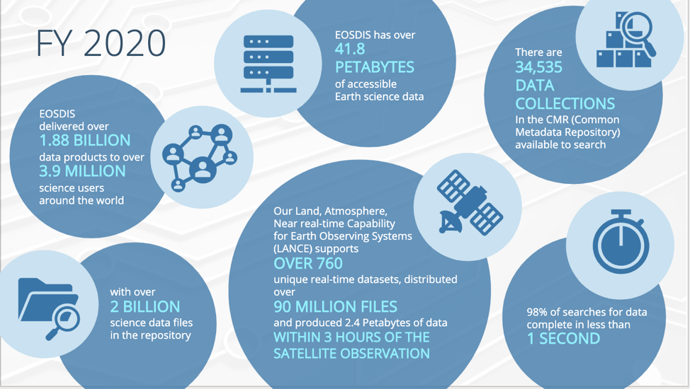
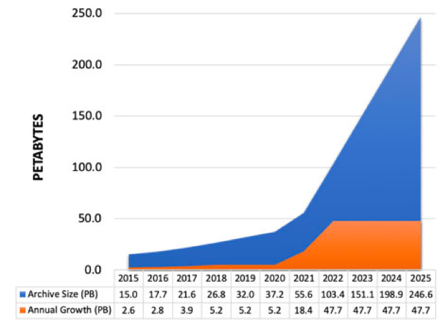
The NASA Earthdata archive continues to grow
EOSDIS Data Archive
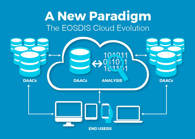
The NASA Earthdata Cloud Evolution
NASA Distributed Active Archive Centers (DAACs) are continuing to migrate data to the Earthdata Cloud
Supporting increased data volume as new, high-resolution remote sensing missions launch in the coming years
Data hosted via Amazon Web Services, or AWS
DAACs continuing to support tools, services, and tutorial resources for our user communities
NASA Earthdata Cloud as an enabler of Open Science
Reducing barriers to large-scale scientific research in the era of “big data”
Increasing community contributions with hands-on engagement
Promoting reproducible and shareable workflows without relying on local storage systems
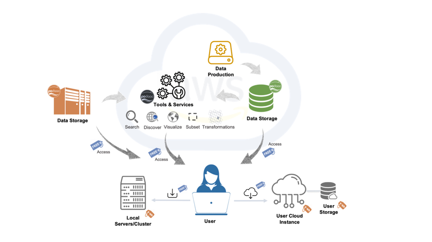
Open Data
Data and Analysis co-located “in place”
Earthdata Cloud Paradigm
Building NASA Earthdata Cloud Resources
Show slide with 3 panels of user resources
Emphasize that the following tutorials are short examples that were taken from the tutorial resources we have been building for our users
NASA Earthdata Cloud: Discovery and access using open source technologies
The following tutorial demonstrates several basic end-to-end workflows to interact with data “in-place” from the NASA Earthdata Cloud, accessing Amazon Web Services (AWS) Single Storage Solution (S3) data locations without the need to download data. While the data can be downloaded locally, the cloud offers the ability to scale compute resources to perform analyses over large areas and time spans, which is critical as data volumes continue to grow.
Although the examples we’re working with in this notebook only focuses on a small time and area for demonstration purposes, this workflow can be modified and scaled up to suit a larger time range and region of interest.
Datasets of interest:
Harmonized Landsat Sentinel-2 (HLS) Operational Land Imager Surface Reflectance and TOA Brightness Daily Global 30m v2.0 (L30) (10.5067/HLS/HLSL30.002)
Surface reflectance (SR) and top of atmosphere (TOA) brightness data
Global observations of the land every 2–3 days at 30-meter (m)
Time series of monthly NetCDFs on a 0.5-degree latitude/longitude grid.
Part 1: Explore Data hosted in the Earthdata Cloud
Earthdata Search Demonstration
From Earthdata Search https://search.earthdata.nasa.gov, use your Earthdata login credentials to log in. You can create an Earthdata Login account at https://urs.earthdata.nasa.gov.
In this example we are interested in the ECCO dataset, hosted by the PO.DAAC. This dataset is available from the NASA Earthdata Cloud archive hosted in AWS cloud.
Click on the “Available from AWS Cloud” filter option on the left. Here, 39 matching collections were found with the ECCO monthly SSH search, and for the time period for year 2015. The latter can be done using the calendar icon on the left under the search box. Scroll down the list of returned matches until we see the dataset of interest, in this case ECCO Sea Surface Height - Monthly Mean 0.5 Degree (Version 4 Release 4).
View and Select Data Access Options
Clicking on the ECCO Sea Surface Height - Monthly Mean 0.5 Degree (Version 4 Release 4) dataset, we now see a list of files (granules) that are part of the dataset (collection). We can click on the green + symbol to add a few files to our project. Here we added the first 3 listed for 2015. Then click on the green button towards the bottom that says “Download”. This will take us to another page with options to customize our download or access link(s).
Figure caption: Select granules and click download
Access Options
Select the “Direct Download” option to view Access options via Direct Download and from the AWS Cloud. Additional options to customize the data are also available for this dataset.
Figure caption: Customize your download or access
Earthdata Cloud access information
Clicking the green Download Data button again, will take us to the final page for instructions to download and links for data access in the cloud. The AWS S3 Access tab provides the S3:// links, which is what we would use to access the data directly in-region (us-west-2) within the AWS cloud.
E.g.: s3://podaac-ops-cumulus-protected/ECCO_L4_SSH_05DEG_MONTHLY_V4R4/SEA_SURFACE_HEIGHT_mon_mean_2015-09_ECCO_V4r4_latlon_0p50deg.nc where s3 indicates data is stored in AWS S3 storage, podaac-ops-cumulus-protected is the bucket, and ECCO_L4_SSH_05DEG_MONTHLY_V4R4 is the object prefix (the latter two are also listed in the dataset collection information under Cloud Access (step 3 above)).
Integrate file links into programmatic workflow, locally or in the AWS cloud.
In the next two examples we will work programmatically in the cloud to access datasets of interest, to get us set up for further scientific analysis of choice. There are several ways to do this. One way to connect the search part of the workflow we just did in Earthdata Search to our next steps working in the cloud is to simply copy/paste the s3:// links provides in Step 4 above into a JupyterHub notebook or script in our cloud workspace, and continue the data analysis from there.
One could also copy/paste the s3:// links and save them in a text file, then open and read the text file in the notebook or script in the JupyterHub in the cloud.
Figure caption: Direct S3 access
Part 2: Working with Cloud-Optimized GeoTIFFs using NASA’s Common Metadata Repository Spatio-Temporal Assett Catalog (CMR-STAC)
In this example we will access the NASA’s Harmonized Landsat Sentinel-2 (HLS) version 2 assets, which are archived in cloud optimized geoTIFF (COG) format archived by the Land Processes (LP) DAAC. The COGs can be used like any other GeoTIFF file, but have some added features that make them more efficient within the cloud data access paradigm. These features include: overviews and internal tiling.
But first, what is STAC?
SpatioTemporal Asset Catalog (STAC) is a specification that provides a common language for interpreting geospatial information in order to standardize indexing and discovering data.
The STAC specification is made up of a collection of related, yet independent specifications that when used together provide search and discovery capabilities for remote assets.
The CMR-STAC API is NASA’s implementation of the STAC API specification for all NASA data holdings within EOSDIS. The current implementation does not allow for querries accross the entire NASA catalog. Users must execute searches within provider catalogs (e.g., LPCLOUD) to find the STAC Items they are searching for. All the providers can be found at the CMR-STAC endpoint here: https://cmr.earthdata.nasa.gov/stac/.
In this example, we will query the LPCLOUD provider to identify STAC Items from the Harmonized Landsat Sentinel-2 (HLS) collection that fall within our region of interest (ROI) and within our specified time range.
Import packages
import osimport requests import boto3from osgeo import gdalimport rasterio as riofrom rasterio.session import AWSSessionimport rioxarrayimport hvplot.xarrayimport holoviews as hvfrom pystac_client import Client from collections import defaultdict import jsonimport geopandasimport geoviews as gvfrom cartopy import crsgv.extension('bokeh', 'matplotlib')
Connect to the CMR-STAC API
STAC_URL ='https://cmr.earthdata.nasa.gov/stac'
provider_cat = Client.open(STAC_URL)
Connect to the LPCLOUD Provider/STAC Catalog
For this next step we need the provider title (e.g., LPCLOUD). We will add the provider to the end of the CMR-STAC API URL (i.e., https://cmr.earthdata.nasa.gov/stac/) to connect to the LPCLOUD STAC Catalog.
catalog = Client.open(f'{STAC_URL}/LPCLOUD/')
Since we are using a dedicated client (i.e., pystac-client.Client) to connect to our STAC Provider Catalog, we will have access to some useful internal methods and functions (e.g., get_children() or get_all_items()) we can use to get information from these objects.
Search for STAC Items
We will define our ROI using a geojson file containing a small polygon feature in western Nebraska, USA. We’ll also specify the data collections and a time range for our example.
Read in a geojson file and plot
Reading in a geojson file with geopandas and extract coodinates for our ROI.
field = geopandas.read_file('../data/ne_w_agfields.geojson')fieldShape = field['geometry'][0]roi = json.loads(field.to_json())['features'][0]['geometry']
We can plot the polygon using the geoviews package that we imported as gv with ‘bokeh’ and ‘matplotlib’ extensions. The following has reasonable width, height, color, and line widths to view our polygon when it is overlayed on a base tile map.
base = gv.tile_sources.EsriImagery.opts(width=650, height=500)farmField = gv.Polygons(fieldShape).opts(line_color='yellow', line_width=10, color=None)base * farmField
We will now start to specify the search criteria we are interested in, i.e, the date range, the ROI, and the data collections, that we will pass to the STAC API.
Search the CMR-STAC API with our search criteria
Now we can put all our search criteria together using catalog.search from the pystac_client package. STAC Collection is synonomous with what we usually consider a NASA data product. Desired STAC Collections are submitted to the search API as a list containing the collection id. Let’s focus on S30 and L30 collections.
Below we will loop through and filter the item_collection by a specified cloud cover as well as extract the band we’d need to do an Enhanced Vegetation Index (EVI) calculation for a future analysis. We will also specify the STAC Assets (i.e., bands/layers) of interest for both the S30 and L30 collections (also in our collections variable above) and print out the first ten links, converted to s3 locations:
cloudcover =25s30_bands = ['B8A', 'B04', 'B02', 'Fmask'] # S30 bands for EVI calculation and quality filtering -> NIR, RED, BLUE, Quality l30_bands = ['B05', 'B04', 'B02', 'Fmask'] # L30 bands for EVI calculation and quality filtering -> NIR, RED, BLUE, Quality evi_band_links = []for i in item_collection:if i.properties['eo:cloud_cover'] <= cloudcover:if i.collection_id =='HLSS30.v2.0':#print(i.properties['eo:cloud_cover']) evi_bands = s30_bandselif i.collection_id =='HLSL30.v2.0':#print(i.properties['eo:cloud_cover']) evi_bands = l30_bandsfor a in i.assets:ifany(b==a for b in evi_bands): evi_band_links.append(i.assets[a].href)s3_links = [l.replace('https://data.lpdaac.earthdatacloud.nasa.gov/', 's3://') for l in evi_band_links]s3_links[:10]
Access s3 credentials from LP.DAAC and create a boto3 Session object using your temporary credentials. This Session is used to pass credentials and configuration to AWS so we can interact wit S3 objects from applicable buckets.
GDAL is a foundational piece of geospatial software that is leveraged by several popular open-source, and closed, geospatial software. The rasterio package is no exception. Rasterio leverages GDAL to, among other things, read and write raster data files, e.g., GeoTIFFs/Cloud Optimized GeoTIFFs. To read remote files, i.e., files/objects stored in the cloud, GDAL uses its Virtual File System API. In a perfect world, one would be able to point a Virtual File System (there are several) at a remote data asset and have the asset retrieved, but that is not always the case. GDAL has a host of configurations/environmental variables that adjust its behavior to, for example, make a request more performant or to pass AWS credentials to the distribution system. Below, we’ll identify the evironmental variables that will help us get our data from cloud
PROJCS["UTM Zone 11, Northern Hemisphere",GEOGCS["Unknown datum based upon the WGS 84 ellipsoid",DATUM["Not_specified_based_on_WGS_84_spheroid",SPHEROID["WGS 84",6378137,298.257223563,AUTHORITY["EPSG","7030"]]],PRIMEM["Greenwich",0],UNIT["degree",0.0174532925199433,AUTHORITY["EPSG","9122"]]],PROJECTION["Transverse_Mercator"],PARAMETER["latitude_of_origin",0],PARAMETER["central_meridian",-117],PARAMETER["scale_factor",0.9996],PARAMETER["false_easting",500000],PARAMETER["false_northing",0],UNIT["metre",1,AUTHORITY["EPSG","9001"]],AXIS["Easting",EAST],AXIS["Northing",NORTH]]
semi_major_axis :
6378137.0
semi_minor_axis :
6356752.314245179
inverse_flattening :
298.257223563
reference_ellipsoid_name :
WGS 84
longitude_of_prime_meridian :
0.0
prime_meridian_name :
Greenwich
geographic_crs_name :
Unknown datum based upon the WGS 84 ellipsoid
horizontal_datum_name :
Not_specified_based_on_WGS_84_spheroid
projected_crs_name :
UTM Zone 11, Northern Hemisphere
grid_mapping_name :
transverse_mercator
latitude_of_projection_origin :
0.0
longitude_of_central_meridian :
-117.0
false_easting :
500000.0
false_northing :
0.0
scale_factor_at_central_meridian :
0.9996
spatial_ref :
PROJCS["UTM Zone 11, Northern Hemisphere",GEOGCS["Unknown datum based upon the WGS 84 ellipsoid",DATUM["Not_specified_based_on_WGS_84_spheroid",SPHEROID["WGS 84",6378137,298.257223563,AUTHORITY["EPSG","7030"]]],PRIMEM["Greenwich",0],UNIT["degree",0.0174532925199433,AUTHORITY["EPSG","9122"]]],PROJECTION["Transverse_Mercator"],PARAMETER["latitude_of_origin",0],PARAMETER["central_meridian",-117],PARAMETER["scale_factor",0.9996],PARAMETER["false_easting",500000],PARAMETER["false_northing",0],UNIT["metre",1,AUTHORITY["EPSG","9001"]],AXIS["Easting",EAST],AXIS["Northing",NORTH]]
GeoTransform :
699960.0 30.0 0.0 4100040.0 0.0 -30.0
array(0)
_FillValue :
-9999.0
scale_factor :
0.0001
add_offset :
0.0
long_name :
Red
When GeoTIFFS/Cloud Optimized GeoTIFFS are read in, a band coordinate variable is automatically created (see the print out above). In this exercise we will not use that coordinate variable, so we will remove it using the squeeze() function to avoid confusion.
PROJCS["UTM Zone 11, Northern Hemisphere",GEOGCS["Unknown datum based upon the WGS 84 ellipsoid",DATUM["Not_specified_based_on_WGS_84_spheroid",SPHEROID["WGS 84",6378137,298.257223563,AUTHORITY["EPSG","7030"]]],PRIMEM["Greenwich",0],UNIT["degree",0.0174532925199433,AUTHORITY["EPSG","9122"]]],PROJECTION["Transverse_Mercator"],PARAMETER["latitude_of_origin",0],PARAMETER["central_meridian",-117],PARAMETER["scale_factor",0.9996],PARAMETER["false_easting",500000],PARAMETER["false_northing",0],UNIT["metre",1,AUTHORITY["EPSG","9001"]],AXIS["Easting",EAST],AXIS["Northing",NORTH]]
semi_major_axis :
6378137.0
semi_minor_axis :
6356752.314245179
inverse_flattening :
298.257223563
reference_ellipsoid_name :
WGS 84
longitude_of_prime_meridian :
0.0
prime_meridian_name :
Greenwich
geographic_crs_name :
Unknown datum based upon the WGS 84 ellipsoid
horizontal_datum_name :
Not_specified_based_on_WGS_84_spheroid
projected_crs_name :
UTM Zone 11, Northern Hemisphere
grid_mapping_name :
transverse_mercator
latitude_of_projection_origin :
0.0
longitude_of_central_meridian :
-117.0
false_easting :
500000.0
false_northing :
0.0
scale_factor_at_central_meridian :
0.9996
spatial_ref :
PROJCS["UTM Zone 11, Northern Hemisphere",GEOGCS["Unknown datum based upon the WGS 84 ellipsoid",DATUM["Not_specified_based_on_WGS_84_spheroid",SPHEROID["WGS 84",6378137,298.257223563,AUTHORITY["EPSG","7030"]]],PRIMEM["Greenwich",0],UNIT["degree",0.0174532925199433,AUTHORITY["EPSG","9122"]]],PROJECTION["Transverse_Mercator"],PARAMETER["latitude_of_origin",0],PARAMETER["central_meridian",-117],PARAMETER["scale_factor",0.9996],PARAMETER["false_easting",500000],PARAMETER["false_northing",0],UNIT["metre",1,AUTHORITY["EPSG","9001"]],AXIS["Easting",EAST],AXIS["Northing",NORTH]]